Brillouin Zones (all content)

Note: DoITPoMS Teaching and Learning Packages are intended to be used interactively at a computer! This print-friendly version of the TLP is provided for convenience, but does not display all the content of the TLP. For example, any video clips and answers to questions are missing. The formatting (page breaks, etc) of the printed version is unpredictable and highly dependent on your browser.

Contents

Main pages

Additional pages

Aims

On completion of this TLP you should:

• Understand how to generate the reciprocal lattice from the real space lattice
• Know how to construct Brillouin Zones in reciprocal space
• Be familiar with the Brillouin Zones for some simple two- and three-dimensional structures

Before you start

Though this package is largely self-contained, some familiarity with simple crystal lattices is useful. If you want a reminder, look at the teaching and learning package on Crystallography and Miller indices and lattice planes.

Introduction

Leon Brillouin (1889-1969) first introduced Brillouin Zones in his work on the general properties of periodic structures. The concept and construction of the zones can appear quite abstract, but this is largely a result of their wide range of useful applications.

Brillouin zones are polyhedra in reciprocal space in crystalline materials and are the geometrical equivalent of Wigner-Seitz cells in real space. Physically, Brillouin zone boundaries represent Bragg planes which reflect (diffract) waves having particular wave vectors so that they cause constructive interference.

Reciprocal lattice vectors

Every periodic structure has two lattices associated with it. The first is the real space lattice, and this describes the periodic structure. The second is the reciprocal lattice, and this determines how the periodic structure interacts with waves. This section outlines how to find the basis vectors for the reciprocal lattice from the basis vectors of the real space lattice.

Reciprocal lattice vectors, K, are defined by the following condition:

$${e^{i{\bf{K}} \cdot {\bf{R}}}} = 1$$

where R is a real space lattice vector. Any real lattice vector may be expressed in terms of the lattice basis vectors, a₁, a₂, a₃.

$${\bf{R}} = {c_1}{{\bf{a}}_{\bf{1}}} + {c_2}{{\bf{a}}_{\bf{2}}} + {c_3}{{\bf{a}}_{\bf{3}}}$$

in which the c_i are integers. The condition on the reciprocal lattice vectors may also be expressed as

$${\bf{K}} \cdot {\bf{R}} = 2\pi .n$$

where n is an integer. This expression can be satisfied if K is expressed in terms of the reciprocal lattice basis vectors b_i, which are defined as

$$\eqalign{ & {{\bf{b}}_{\bf{1}}} = {{2\pi \cdot {{\bf{a}}_{\bf{2}}} \times {{\bf{a}}_{\bf{3}}}} \over {\left| {{{\bf{a}}_{\bf{1}}} \cdot {{\bf{a}}_{\bf{2}}} \times {{\bf{a}}_{\bf{3}}}} \right|}} \cr & {{\bf{b}}_{\bf{2}}} = {{2\pi \cdot {{\bf{a}}_{\bf{3}}} \times {{\bf{a}}_{\bf{1}}}} \over {\left| {{{\bf{a}}_{\bf{1}}} \cdot {{\bf{a}}_{\bf{2}}} \times {{\bf{a}}_{\bf{3}}}} \right|}} \cr & {{\bf{b}}_{\bf{3}}} = {{2\pi \cdot {{\bf{a}}_{\bf{1}}} \times {{\bf{a}}_{\bf{2}}}} \over {\left| {{{\bf{a}}_{\bf{1}}} \cdot {{\bf{a}}_{\bf{2}}} \times {{\bf{a}}_{\bf{3}}}} \right|}} \cr} $$

Note that b₂ and b₃ are given by cyclic permutations of the expression for b₁ . From this expression it may be seen that the real lattice basis vectors and the reciprocal lattice basis vectors satisfy the following relation:

$${{\bf{b}}_i} \cdot {{\bf{a}}_j} = 2\pi {\delta _{ij}}$$

where \({\delta _{ij}}\)>is the Kronecker delta, which takes the value 1 when i is equal to j, and 0 otherwise. Any reciprocal lattice vector may then be expressed as a linear sum of these reciprocal basis vectors:

$${\bf{K}} = h{{\bf{b}}_{\bf{1}}} + k{{\bf{b}}_{\bf{2}}} + l{{\bf{b}}_{\bf{3}}}$$

in which h, k and l are integers. The set of all K vectors defines the reciprocal lattice.

Brillouin Zone construction

The reciprocal lattice basis vectors span a vector space that is commonly referred to as reciprocal space, or often in the context of quantum mechanics, k space. This section covers the construction of Brillouin zones in two dimensions.

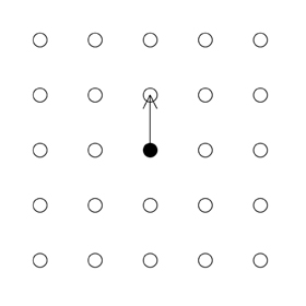
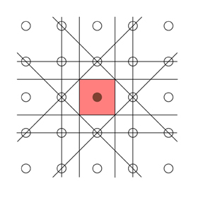
The first step is to use the real space lattice vectors to find the reciprocal lattice vectors and construct the reciprocal lattice. One of the points in the reciprocal lattice is then designated to be the origin. When constructing Brillouin zones, they are always centred on a reciprocal lattice point, but it is important to keep in mind that there is nothing special about this point as each reciprocal lattice point is equivalent due to translation symmetry.

Draw a line connecting this origin point to one of its nearest neighbours. This line is a reciprocal lattice vector as it connects two points in the reciprocal lattice.

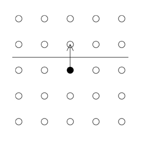
Then draw on a perpendicular bisector to the first line. This perpendicular bisector is a Bragg Plane.

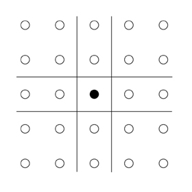
Add the Bragg Planes corresponding to the other nearest neighbours.

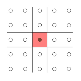
The locus of points in reciprocal space that have no Bragg Planes between them and the origin defines the first Brillouin Zone. It is equivalent to the Wigner-Seitz unit cell of the reciprocal lattice. In the picture below the first Zone is shaded red.

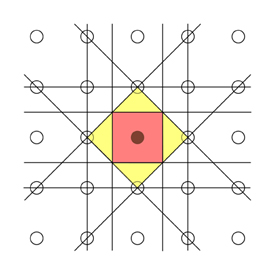
Now draw on the Bragg Planes corresponding to the next nearest neighbours.

The second Brillouin Zone is the region of reciprocal space in which a point has one Bragg Plane between it and the origin. This area is shaded yellow in the picture below. Note that the areas of the first and second Brillouin Zones are the same.

The construction can quite rapidly become complicated as you move beyond the first few zones, and it is important to be systematic so as to avoid missing out important Bragg Planes. Click the animation below for an interactive illustration that follows this process to show how to construct the first six Brillouin Zones for the 2-D square reciprocal lattice. Use the arrow buttons to navigate forwards and backwards through the different steps.

2-D square lattice

As a further example, click the on the animation below for an interactive illustration showing how to construct the first six zones for a 2-D hexagonal reciprocal lattice.

2-D hexagonal lattice

The general case in three dimensions

After considering these simple examples, it should hopefully be clear how to construct Brillouin Zones. Whilst in two dimensions this geometric method is easy to apply, in three dimensions the lattice cannot be represented on a piece of paper and in general it is much harder to picture the shape of the Brillouin Zones beyond the first. This section considers how the relevant Bragg planes for zone construction may be generated in a systematic fashion.

In vector notation, the equation of a plane may be written as

$${\bf{(r}} - {\bf{a)}} \cdot {\bf{\hat n}} = 0$$

In this expression, a is a vector from the origin to a specified (but arbitrary) point in the plane, r is a general point in the plane and \({\bf{\hat n}}\) is the unit vector normal to the plane.

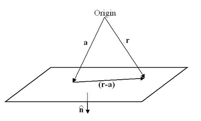
For Brillouin Zones it is convenient to choose a so that it is the perpendicular vector from the origin to the Bragg plane of interest, i.e., a vector of the form

$${\bf{a}} = {1 \over 2}(h{{\bf{b}}_{\bf{1}}} + k{{\bf{b}}_{\bf{2}}} + l{{\bf{b}}_{\bf{3}}})$$

also, the unit normal is then given by \({\bf{\hat n}} = {{\bf{a}} \over {\left| {\bf{a}} \right|}}\)

Letting h, k and l be integers (positive or negative) and excluding the point where all three are equal to zero, the relevant Bragg Planes may be generated in a systematic fashion. It is usually sufficient for finding the first three or four zones to have the d_i range between –3 and +3.

Then, given any point in reciprocal space, it may be allocated to a Brillouin zone by determining the number, N, of Bragg Planes that lie in between that point and the origin. The point is then in the (N+1)th Brillouin Zone.

Whether a Bragg plane lies between a general point, r, and the origin may be determined quite simply by considering the projection of the position vector of the point in the direction of the unit normal to the Bragg plane. The scalar product

a.(r – a)

is positive if the plane is between the point and the origin, and is negative when the plane does not lie between the point and the origin.

The main complication when extending to Brillouin Zones beyond the first zone is that it is very easy to overlook an important Bragg Plane. This can only really be avoided by being careful and systematic. A useful test to indicate if a mistake has been made is to check that all the zones have the same symmetries as the reciprocal lattice itself. For example the Brillouin Zones for the 2-D Square lattice always have fourfold-rotational symmetry about the origin. A further useful check is to confirm that the area (in 2D) or volume (in 3D) of each Brillouin zone is the same.

Some examples which show the Brillouin Zones for common 2-D lattices may be found by clicking the links below.

• 2-D Square lattice to 10th Brillouin zone (pdf file, 0.53 MB)
• 2-D Hexagonal lattice to 6th Brillouin zone (pdf file, 0.60 MB)
  

Zone folding

An important property of the Brillouin Zones is that, because the reciprocal lattice is periodic, there exists for any point outside the first zone a unique reciprocal lattice vector that will translate that point back inside the first zone. Each point in reciprocal space is only unique up to a reciprocal lattice vector. Each Zone contains every single physically distinguishable point, and so they all have the same area (in 2-D) or volume (in 3-D).

This is easiest to see by example. The links below are for interactive illustrations which will show how the first six zones for the 2-D square and hexagonal lattices can be translated or 'folded' back on top of the first zone. Use the arrow buttons to navigate through the different steps.

2-D square Zone folding

2-D hexagonal Zone folding

Examples of Brillouin Zones in Three Dimensions

The extension to three dimensions is straightforward by the method outlined in the previous section. However, it is important to remember not to overlook important Bragg Planes. There is also a problem of representation, because the structure of the Zones in 3-D can be quite complicated and hard to visualise.

It is also important to remember that in 3-D the Zones all have the same volume, and that the volume corresponding to the 3rd Zone is the volume between the outer surface of the 2nd Zone and that of the 3rd Zone.

Representations of the Brillouin Zones corresponding to Simple Cubic (SC), Body Centred Cubic (BCC), Face Centred Cubic (FCC) lattices are linked to below. Use the buttons on the left hand side to select which Zone Surface to view, and use the arrow buttons to rotate the view about the [001] axis.

Simple Cubic

Body Centred Cubic

Face Centred Cubic

Summary

This teaching and learning package has introduced Brillouin zones and their construction in two and three dimensions.

The relationship between the construction of Brillouin zones and diffraction from Bragg Planes has been shown by a consideration of the Bragg equation.

The examples shown in the package itself demonstrate the principles of the construction in two dimensions. In three dimensions the principles of the construction are the same, but the Brillouin Zones are hard to visualise. Rotating the shapes of Brillouin Zones about a cube axis as in the examples we have given in this package helps to improve the visualisation in comparison with simple line diagrams found in textbooks.

Questions

Quick questions

You should be able to answer these questions without too much difficulty after studying this TLP. If not, then you should go through it again!

1. If a real space vector has length L, what is the magnitude of the corresponding reciprocal lattice vector as defined in this TLP?

   	a
   	b
   	c
   	d

2. Which of the following statements about the Brillouin zones for a particular reciprocal lattice are correct? (select yes for true and no for false for each statement)

   Yes	No	a	They all have the same area / volume.
   Yes	No	b	They all have the same shape.
   Yes	No	c	They all have the same symmetry.

Deeper questions

The following questions require some thought and reaching the answer may require you to think beyond the contents of this TLP.

3. By either printing out the lattice in the file linked to here (pdf), or by drawing out a rectangular lattice with the ratio between the short and long sides of 4:5. Use the method outlined earlier to construct the first three Brillouin zones, being careful not to miss any relevant Bragg planes.

4. By either printing out the lattice in the file linked to here (pdf), or by drawing out a parallelogram lattice with the ratio between the short and long sides of 4:5 and an angle between the sides of about 75 degrees. Use the method outlined earlier to construct the first three Brillouin zones, being careful not to miss an relevant Bragg planes.

5. Confirm that when expressed in a Cartesian basis, possible lattice vectors of the primitive unit cell (i.e., the unit cell with one lattice point per unit cell) for a FCC lattice of unit side length are , and .

6. Confirm that when expressed in a Cartesian basis, possible lattice vectors of the primitive unit cell for a BCC lattice of unit side length are , and .

7. Using the definition of the reciprocal lattice basis vectors given in the TLP, show that the reciprocal lattice of a FCC lattice is a BCC lattice and vice versa.

8. For a conventional BCC unit cell with two lattice points per unit cell of side L:

   1. How many nearest neighbours does each point have?
   2. What are their coordinates, and what distance away are they?
   3. How many next nearest neighbours are there?
   4. What are their coordinates and what distance away are they?

9. Look at the picture below of the first Brillouin zone for a real space FCC lattice. Using your answers to questions 5 and 6, try to index the planes labelled (a) and (b).

   

Going further

Books

There a number of textbooks which discuss in varying levels of detail Brillouin Zones and their construction and application. The classic text on Brillouin Zones is

• Wave Propagation in Periodic Structures, L. Brillouin (Dover 1953, reprinted 2003)

Other texts are also useful, such as:

• Solid State Physics, J.S. Blakemore (Saunders 1974)
• Electronic Properties of Materials, R.E. Hummel (Springer-Verlag 1992)
• Introduction to Solid State Physics, C. Kittel (Wiley 1996)
• Solid State Physics, N.W. Ashcroft and N. D. Mermin. (Harcourt Brace 1976)

Websites

• Wikipedia - Brillouin zones
  This wikipedia page has a number of useful external links which should help to reinforce and confirm the concepts introduced in this teaching and learning package.

Further links can be readily found by typing “Brillouin Zones” into Google and searching the web. Examples of such links are:

• http://www.tf.uni-kiel.de/matwis/amat/semi_en/kap_2/illustr/i2_1_3.html
• http://britneyspears.ac/physics/crystals/wcrystals.htm

Bragg planes and Brillouin zone construction

The construction of Bragg Planes in the context of Brillouin zones can be understood by considering Bragg’s Law

λ = 2dsinθ

where θ is the angle between the incident radiation and the diffracting plane, λ is the wavelength of the incident radiation and d is the interplanar spacing of the diffracting planes. (Further information on Bragg’s Law is found in the TLP on X-ray diffraction).

In reciprocal space this can be expressed in the form

k' – k = g

where k is the wave vector of the incident wave of magnitude 2π/λ, k' is the wave vector of the diffracted wave, also of magnitude 2π/λ, and g is a reciprocal lattice vector of magnitude 2π/d:

This can be shown graphically using the Ewald sphere construction:

Here 000 is the origin of the reciprocal lattice and O is the centre of the sphere of radius \(\left| {\bf{k}} \right|{\rm{ }}\). If the angle subtended at O between 000 and G on the above diagram is 2θ, simple geometry shows that

\[\sin \theta = {{\left| {\bf{g}} \right|} \over {2\left| {\bf{k}} \right|}} = {{{{2\pi } \over {{d_{hkl}}}}} \over {2.{{2\pi } \over \lambda }}} = {\lambda \over {2{d_{hkl}}}}\]

which can be rearranged into the more familiar form

\[\lambda = 2{d_{hkl}}\sin \theta \]

i.e., the Bragg equation.

The equation

k' – k = g

can be rearranged in the form

k' = k + g

Hence

k'.k' = (k + g).(k + g) = k.k + g.g + 2k.g

Since k'.k' = k.k because diffraction is an elastic scattering event, it follows that

g.g + 2k.g = 0

To construct the Bragg Plane, it is convenient to replace k by -k in this equation so that both k and g begin at the origin, 000, of the reciprocal lattice. Hence, the equation can be written in the form

\[{\bf{k}}.\left( {{1 \over 2}{\bf{g}}} \right) = \left( {{1 \over 2}{\bf{g}}} \right).\left( {{1 \over 2}{\bf{g}}} \right)\]

Constructing the plane normal to g at the midpoint, \({1 \over 2}{\bf{g}}\), then means that any vector k drawn from the origin, 000, to a position on this plane satisfies the Bragg diffraction condition:

Academic consultant: Kevin Knowles (University of Cambridge)
Content development: Chris Dunleavy
Web development: Lianne Sallows

This DoITPoMS TLP was funded by the UK Centre for Materials Education and the Department of Materials Science and Metallurgy, University of Cambridge.

Additional support for the development of this TLP came from the Worshipful Company of Armourers and Brasiers'