Solidification of Alloys (all content)
Note: DoITPoMS Teaching and Learning Packages are intended to be used interactively at a computer! This print-friendly version of the TLP is provided for convenience, but does not display all the content of the TLP. For example, any video clips and answers to questions are missing. The formatting (page breaks, etc) of the printed version is unpredictable and highly dependent on your browser.
Contents
Main pages
Additional pages
Aims
On completion of this TLP you should:
- Know how limited diffusion in the solid and liquid phases affects the distribution of solute in a solidified alloy, and be able to predict these effects in certain samples.
- Understand the factors that control the shape of a solid growth front, and the resulting microstructure.
Before you start
You should understand phase diagrams, and how they can be used to predict the form of a solidified alloy. It would also be helpful to have an understanding of (Fick's first law of diffusion and Fick's second law of diffusion ). You might want to look at the TLPs on Diffusion, Phase Diagrams and Solidification, and Solid Solutions,
Introduction
Metals and alloys are almost always cast from a liquid at some point during the manufacturing process, as they are typically obtained from their ores in liquid form, or melted down from scrap. Also, alloying two or more elements is usually done in the liquid phase, because rapid diffusion is required to ensure a uniform composition. This means that an understanding of how metals and alloys solidify is essential to allow us to explain and control the properties of the solid that is formed.
Solute Partitioning
The TLP Phase Diagrams and Solidification explains the method for determining the concentrations and proportions of the phases formed in solidification of a binary alloy , from the phase diagram, assuming that equilibrium can be achieved, and the most thermodynamically favourable phases formed. This method is known as the lever rule.
Consider the case of a binary alloy, Al-5wt%Cu:
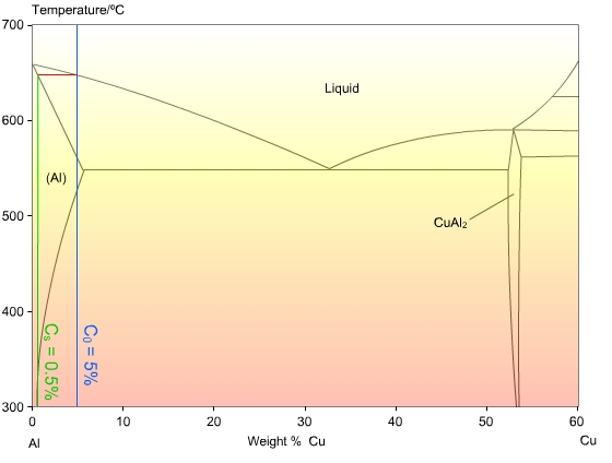
The phase diagram shows that the first solid formed, CS, at 650 °C, will be 0.5 wt%Cu, but the stable phase after total solidification is a complete solid solution with a concentration of 5 wt%Cu. Clearly there will need to be significant diffusion in the solid to allow the solute to distribute evenly, and for equilibrium to occur.
This diffusion can be described mathematically by Fick’s laws:
\[J = - D\left( {\frac{{\partial C}}{{\partial x}}} \right)\]
\[\left( {\frac{{\partial C}}{{\partial t}}} \right) = D\left( {\frac{{{\partial ^2}C}}{{\partial {x^2}}}} \right)\]
The self diffusion coefficient in the solid phase, Ds, varies from about 10-10 to 10-14 m2 s-1 at the melting point, depending on the material in question, and also obeys Arrhenius’ equation for temperature dependency:
\[D = {D_0}\exp \left( {\frac{{ - Q}}{{RT}}} \right)\]
Values of diffusivity in most liquid metals are significantly higher, of the order of 10-9 m2 s-1, but also obey Arrhenius’ law.
The graph below shows how the self-diffusivity (diffusivity ) , D, varies with the undercooling below the melting temperature, Tm, in copper.
The interdiffusivity (diffusivity ) in the alloy will behave in a similar way, so we can see that unless the alloy is cooled very slowly, the diffusivity will drop off rapidly before significant diffusion can occur into the solid, resulting in “coring” of grains, with lower solute concentration at the centre, where the first solid formed; and higher solute concentration at the edges. If the solute partitioning is extensive enough to raise the concentration of the liquid to the eutectic composition (eutectic ) the remaining liquid will then freeze with that composition in a eutectic structure, as in the micrograph of an Al-5 wt% Cu (5% copper, and 95% aluminium, by weight) alloy shown below:
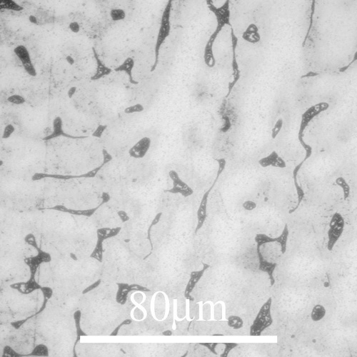
The pale areas are dendrites with a structure based on Al, getting darker towards the edges as the Cu concentration increases. The dark areas are the eutectic that forms in between the dendrites as fine lamellae of Al and CuAl2.
In order to obtain quantitative expressions for the way solute is distributed, we need to use a quantity known as the partition coefficient, k, given by:
\[k = \frac{{{C_S}}}{{{C_L}}}\]
This is the ratio of the concentrations at the solidus , and liquidus , CL, at a given temperature. It determines the extent to which solute is ejected into the liquid during solidification. If the solidus and liquidus are straight lines, then k is independent of temperature. The calculation of k is shown in the Bi-Sn phase diagram below:
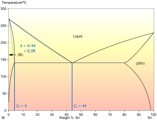
In most cases, the liquidus and solidus are not straight lines, but they are often close enough that we can assume that k is independent of temperature. Also, it is often the case that k is less than one, so that the solid forming is of a higher purity than the liquid.
The Scheil Equation
Since the properties of an alloy can depend strongly on the concentration of solutes that it contains, being able to quantitatively predict the concentrations in the solid is desirable, but a mathematical description of solidification is very difficult in the general case. Solutions can be obtained when certain assumptions are made. For example, we can assume:
- There is no diffusion the solid phase, DS = 0. This will hold if the characteristic diffusion distance is much smaller than the length of the sample, \(\sqrt {{D_{\rm{S}}}t} \) << L
- There is complete mixing in the liquid phase, giving a uniform concentration in the liquid. This may occur because of convection, or can be aided by mechanical mixing.
Using these assumptions we can derive the Scheil equation, which describes the composition of the solid and liquid during solidification, as a function of the fraction solidified. Work through the animation to see how the conditions required to derive the Scheil equation are obtained:
Equating the amount of solute in the shaded areas gives:
( CL - Cs ) df = ( 1 - f ) dC
Solving this gives us the Scheil equation, for the profile of solute in the completely solidified bar:
Cs = k C0 ( 1 - fs )k-1
where CS is the concentration of solute in the solid, at a fractional distance along the bar, fS, C0 is the initial concentration of the liquid, and k is the partition coefficient.
To see a full derivation of the equation, click here.
The Scheil equation predicts a profile with a concentration that tends towards infinity at the end of the bar, but clearly there will be an upper limit on the concentration of any solid forming. In the case where A and B form a complete solid solution across the composition range, the liquid will, at some point, reach a concentration of 100 %B and hence solidify as pure B. An alternative case arises in a binary eutectic system of A and B, where a solid eutectic structure will form when the concentration of the liquid reaches the eutectic concentration.
Steady State Solidification
We can also consider another situation, where there is still no diffusion in the solid phase, but in the liquid phase there is now limited diffusion, rather than complete mixing.
From Fick’s second law, we have:
\[\frac{{{\rm{d}}C}}{{{\rm{d}}t}} = {D_{\rm{L}}}\frac{{{{\rm{d}}^2}C}}{{{\rm{d}}{x^2}}}\]
also:
\[\frac{{{\rm{d}}C}}{{{\rm{d}}t}} = \frac{{{\rm{d}}C}}{{{\rm{d}}x}}\frac{{{\rm{d}}x}}{{{\rm{d}}t}} = v\left( {\frac{{{\rm{d}}C}}{{{\rm{d}}x}}} \right)\]
These combine to give:
\[{D_{\rm{L}}}\left( {\frac{{{{\rm{d}}^2}C}}{{{\rm{d}}{x^2}}}} \right) + v\left( {\frac{{{\rm{d}}C}}{{{\rm{d}}x}}} \right) = 0\]
which can be evaluated with the appropriate boundary conditions to give us:
\[C = {C_0} + \frac{{{C_0}\left( {1 - k} \right)}}{k}\exp \left( {\frac{x}{{{D_{\rm{L}}}/v}}} \right)\]
This equation describes the solute profile in the liquid ahead of the interface, in the steady state. For a full derivation, click here. In the following pages, x should, strictly speaking, be written everywhere as x’ (distance ahead of the moving front)
This model describes the solute profile in the liquid ahead of the interface once the situation has reached a steady state. However, when solidifying a bar, for example; it will take a period of time for the solute ‘bow wave’ to build up ahead of the interface. During this initial transient solid will be forming with a concentration less than C0, (initially it will be k C0) until a steady state is achieved. The solid then advances along the length of the bar with the solute bow wave ahead of the interface. When the bow wave, with a characteristic length, DL / v, begins to run into the end of the bar, the solute ‘piles up’ giving a rapid increase in the solute concentration of the liquid. This final transient sees an increase in the concentration of the solid, and may result in the formation of some non-equilibrium eutectic at the end of the bar.
The simulation below uses a numerical model to predict the solute profiles for the solidification of a 10 mm bar, with a bulk concentration of 10 %. The partition coefficient, k, the size of the solute bow wave; which is dictated by DL/v, and the eutectic composition for the system can all be changed using the scroll bars.
Adjust the variables to see how they each affect the solute profile, and consider why the simulation responds as it does.
Click ‘Run’ to see how the solute profile develops during this schematic movie of steady state solidification.
Zone Refining
Zone refining is an industrial process which makes use of the fact that a material often solidifies with a higher purity than the surrounding liquid, in order to produce materials of very high purity. A bar is passed through a furnace that melts a small section of the bar. As the bar passes through the furnace, this section of liquid is passed along the length of the bar. The solid that forms as the section passes by is of a higher purity than the liquid, and the excess solute is partitioned into the liquid section. After one run, the solute profile will be similar to that after steady state solidification, as the limited size of the liquid section has the same effect as limiting the diffusion in the liquid. Subsequent runs will carry more of the solute to the end of the bar. After many cycles, almost all of the impurity will be concentrated at one end of the bar, which can then be removed, leaving a material of very high purity. Sketches of the solute profile of an initially homogeneous bar, which has been zone refined, are shown after one cycle (left) and many cycles (right).
 |
 |
This process is used in the production of silicon for use in the manufacture of microelectronic devices. The semi-conducting properties of silicon are highly dependent on the type and concentration of dopant atoms; so all impurities have to be removed before any dopants are added.
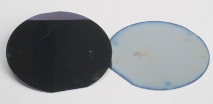
This picture shows the polished (left) and unpolished surfaces of silicon wafers cut from a bar that has been purified by zone refining.
DoITPoMS standard terms of use
Dendritic Growth
The animation below shows how the temperature gradient in the liquid affects the morphology of the growth front in a pure metal:
The animation referred to the driving force for solidification, which is greater for larger undercoolings. To see why, click here.
When a dendritic structure forms, the dendrite arms grow parallel to the favourable growth directions, normally 〈 100 〉 in cubic metals. Grains which are orientated with the 〈 100 〉 direction close to the direction of heat flow will grow fastest and stifle the growth of other grains, leading to a columnar microstructure. To see more about how a microstructure develops in a casting, see the microstructure of a cast ingot section of the TLP on Casting.
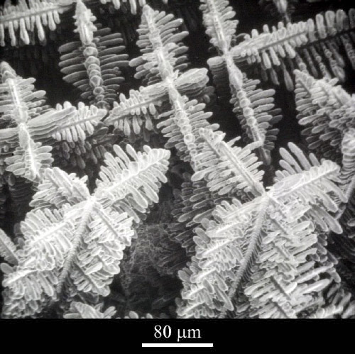 |
This micrograph (left) is an image of the 3D structure of dendrites in a cobalt-samarium-copper alloy, taken with a scanning electron microscope . |
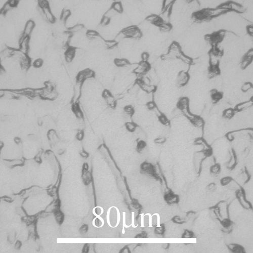
| This micrograph (right), taken with a reflected light microscope, shows the appearance of dendrites of a copper-tin alloy when observed as a 2D section through the 3D structure. | 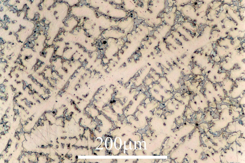 |
Constitutional Undercooling
It is actually rare to have a negative temperature gradient ahead of the interface, yet it is observed that dendrites are very hard to avoid in practice. This occurs because most materials in use have significant levels of impurities. The following animation shows how dendrites form in a binary alloy:
The situation can be analysed quantitatively to determine whether a dendritic growth front is likely. If we assume a steady state diffusion profile ahead of the interface (see page on Steady State Solidification), the concentration of solute at any distance, x’, ahead of the interface is given by:
\[C = {C_0} + \frac{{{C_0}\left( {1 - k} \right)}}{k}\exp \left( {\frac{{ - x}}{{{D_{\rm{L}}}/v}}} \right) \;\;\;\;\;\;(1)\]
The liquidus temperature, TL, on the phase diagram is dependent on the concentration of solute by the equation:
\[{T_{\rm{L}}} = {T_{\rm{m}}} + C\frac{{\partial {T_{\rm{L}}}}}{{\partial C}}\]
where Tm is the melting temperature of the pure substance, and ∂T / ∂x is the gradient of the liquidus on the phase diagram, which is usually negative if k < 1.
The graph of liquidus temperature against distance, has a profile like the one shown below:
There will be an undercooled region ahead of the interface, in which a planar interface is unstable, if the temperature gradient, ∂T / ∂x, ahead of the interface is less than the gradient of the liquidus temperature at the interface. To maintain a planar interface the relationship below must hold:
\[\frac{{\partial T}}{{\partial x}} > {\left. {\frac{{\partial {T_{\rm{L}}}}}{{\partial x}}} \right|_{x = 0}}\]
which, by the chain rule becomes:
\[\frac{{\partial T}}{{\partial x}} > \frac{{\partial {T_{\rm{L}}}}}{{\partial C}}{\left. {\frac{{\partial C}}{{\partial x}}} \right|_{x = 0}}\]
By differentiating (1) with respect to x, and setting x = 0, we get:
\[{\left. {\frac{{\partial C}}{{\partial x}}} \right|_{x = 0}} = - \frac{{{C_0}}}{{{D_{\rm{L}}}/v}}\frac{{\left( {1 - k} \right)}}{k}\]
The critical gradient required to maintain a planar interface is given by:
\[{\frac{{\partial T}}{{\partial x}}_{{\rm{crit}}}} = - \frac{{{C_0}}}{{{D_{\rm{L}}}/v}}\frac{{\left( {1 - k} \right)}}{k}\frac{{\partial {T_{\rm{L}}}}}{{\partial C}}\]
For temperature gradients only slightly below the critical gradient, the planar interface will break down, but the trapping of solute partitioned between the primary dendrite arms prevents growth of secondary arms, and a cellular growth front evolves.
The simulation below allows you to predict the morphology of the solid growth in various systems.
The next simulation plots the liquidus temperature, in black, against distance, on the lower chart. This is calculated from the composition of the liquid, which is plotted on the upper chart. The simulation also plots a temperature profile in the liquid, in red. The gradient of this can be changed using the scrollbar labelled ∂T / ∂x. The upper limit of this gradient is 10000 K m-1, which is an approximate upper limit for gradients that can be practicably achieved. The critical gradient required to ensure a planar interface is plotted in green, and is also displayed in the box. The partition coefficient, k, the bulk concentration, C0, the diffusivity in the liquid DL, and the growth front velocity, v, can all be adjusted using the appropriate scrollbars.
Try adjusting the variables to see how the critical gradient, and the liquidus temperature profile change. Use the appropriate equations to justify the behaviour of the simulation.
You should note that in order to ensure a planar interface, the growth front velocities need to be quite low, of the order of 10s of microns per second. This is why it is often difficult to avoid dendritic growth in practical solidification.
In dendritic growth, most of the solute is ejected between the dendrite arms. The structure of the dendrites serves to prevent mixing with the rest of the liquid, so that the solute partitioning described earlier occurs over the length scale of the secondary dendrite arm spacing. This is known as microsegregation.
Summary
In most cases of solidification, the material is cooled too quickly to allow the equilibrium phases, predicted by the phase diagram, to form. This is because the material does not spend sufficient time at high temperatures where diffusion is faster. The non-equilibrium phases that result can be explained qualitatively by using the phase diagram to predict the composition of the first solid formed. When diffusion is not sufficient for the first solid formed to reach the equilibrium composition, this will result in an excess of solute in the last solid formed, which is often sufficient to cause the formation of a non-equilibrium eutectic.
Quantitative analysis also allows us to predict the compositions of the solid and liquid as a material solidifies, if we assume complete mixing in the liquid and no diffusion in the solid (Scheil equation), or if we assume finite diffusion in the liquid and no diffusion in the solid (Steady state solidification).
We can qualitatively understand the reasons why a planar solidification front breaks down into cells or dendrites, from the fact the solute is partitioned into the liquid at the interface, and any random protuberance will be in a liquid of lower solute concentration, therefore favouring its growth compared to the rest of the solid.
Using the knowledge of the solute profile in the liquid, we can quantitatively predict when dendrites will form as a result of this constitutional undercooling, and also make predictions about the scale and morphology of the structure formed.
Questions
Quick questions
You should be able to answer these questions without too much difficulty after studying this TLP. If not, then you should go through it again!
-
What might cause a material not to form the phases predicted in the phase diagram after solidification?
-
Which assumptions must you make for the Scheil equation to be valid? (You may select more than one answer)
-
When solidifying a hypoeutectic alloy, during which stage of solidification might you form solid with a eutecticstructure?
-
Which of the following reduce the likelihood of dendrites forming in a binary alloy? (You may select more than one answer)
Deeper questions
The following questions require some thought and reaching the answer may require you to think beyond the contents of this TLP.
-
A bar of magnesium is contaminated with aluminium, at a concentration of 2 wt%. The maximum acceptable concentration is 1 wt%. It is to be purified by directional solidification with a planar growth front, and complete mixing in the liquid. Use the Al-Mg interactive phase diagram to estimate the fraction of the bar that will have an acceptable purity.
-
How would the solute profile of a bar, solidified with complete mixing in the liquid, be affected if some diffusion could occur in the solid?
-
An Al-5wt%Cu alloy undergoes steady state solidification, with a growth front velocity of 10 μm s-1. The diffusivity in the liquid is 10-8 m2 s-1. The equipment being used is capable of applying a temperature gradient of up to 104 K m-1, is it possible to ensure that the alloy will solidify with a planar growth front?
- Use the equation:
 to determine the critical temperature gradient in the liquid.
 - The partition coefficient, k, and the liquidus gradient,
 , can be calculated from the phase diagram. (You will need to approximate the liquidus as a straight line.)
- Use the equation:
Open-ended questions
The following questions are not provided with answers, but intended to provide food for thought and points for further discussion with other students and teachers.
-
The micrograph shows a Cu-30wt%Ni alloy that has been chill cast (cast in a mould that is kept much colder than the fusion temperature of the alloy).
Look at the phase diagram, and rationalise the features present in the sample. What is the approximate length scale of the microsegregation in the sample?
The grain structure is dendritic, with primary arm widths of ~20 mm. The formation of dendrites has been caused by constitutional undercooling, which would be unavoidable in chill casting because the high cooling rate means that the growth front velocity is very high.
There is microsegregation, with nickel rich regions showing up pale, and regions lower in nickel appearing darker. The phase diagram shows that the system has a partition coefficient greater than one, so the first solid formed is nickel rich (more impurity), and the final solid to form, between the dendrites is low in nickel. The length scale of the microsegregation is approximately 5 mm.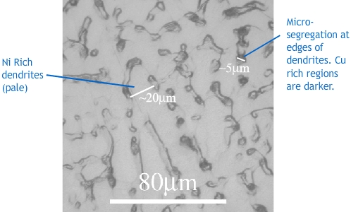
Going further
Books
D. A. Porter and K. E. Easterling, Phase Transformations in Metals and Alloys, Chapman and Hall, 1992.
Chapter 4 covers solidification. Earlier chapters cover phase diagrams, diffusion, and microstructure. Later chapters cover solid-state transformations.
Websites
Matter module: Solidification
This website covers much of the same material as this TLP, but also has more content covering the kinetics of solidification, and the formation of a eutectic structure.
Dendritic solidification
This page covers dendritic solidification, and contains many images of dendrites. The page links to a selection of movies showing dendritic solidification.
Steady State Solute Profile ahead of an Advancing Solidification Front
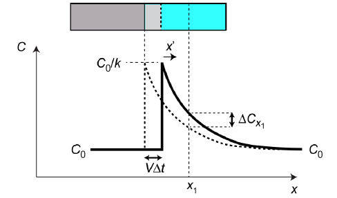
Fig.1 Changing profile during incremental advance of the interface, in a fixed frame (x).
During a time interval Δt, the front advances by VΔt, where V is its velocity. There is no change in the coordinates of physical matter in the fixed frame (neglecting the effect of the volume change on freezing). Any particular slice of liquid, eg at x = x1, will therefore change in composition only as a result of diffusion (governed by the diffusion equation).
$${{\partial C} \over {\partial t}} = D{{{\partial ^2}C} \over {\partial {x^2}}}$$
so that, in time Δt,
$$\Delta {C_{{x_1}}} = \Delta tD{\left. {{{{\partial ^2}C} \over {\partial {x^2}}}} \right|_{x = {x_1}}}$$
Since the profile is in steady state, when referred to the moving frame x’ (= x – Vt), the composition must be constant for all values of x’. This requires
$${\left. {{{\partial C} \over {\partial x}}} \right|_{x = {x_1}}} = {{\Delta {C_{{x_1}}}} \over {\left( { - V\Delta t} \right)}}$$ $$ ∴ - V\Delta t{\left. {{{\partial C} \over {\partial x}}} \right|_{x = {x_1}}} = \Delta tD{\left. {{{{\partial ^2}C} \over {\partial {x^2}}}} \right|_{x = {x_1}}}$$ $${\rm{i}}{\rm{.e}}{\rm{. }}\;D{{{\partial ^2}C} \over {\partial {x^2}}} + V\left( {{{\partial C} \over {\partial x}}} \right) = 0\;\;\;{\rm{for\;\;all\;\;x}}$$
Since x’ is given by (x – Vt), this equation must also hold in the x’ frame.
A solution is now required to this equation that satisfies the boundary conditions. Integrating
$$D\left( {{{\partial C} \over {\partial {x{^′}}}}} \right) = - VC +{\rm{const}}$$
This constant is found by equating the rate of rejection of solute across the interface to the rate at which it is diffusing down the concentration gradient at x’ = 0.
$$D{\left. {{{\partial C} \over {\partial {x^′}}}} \right|_{x = 0}} = - \left( {{{{C_0}} \over k} - {C_0}} \right)V$$ $$ ∴ - \left( {{{{C_0}} \over k} - {C_0}} \right)V + V\left( {{{{C_0}} \over k}} \right) = {\rm{const}}$$
∴ const = V C0
The resultant equation is then integrated again
$$D\left( {{{\partial C} \over {\partial {x^′}}}} \right) = - V(C - {C_0})$$ $${{\partial C} \over {(C - {C_0})}} = - {V \over D}\partial {x^′}$$ $$\ln (C - {C_0}) = - \left( {{V \over D}} \right){x^′} + {\rm{const}}$$
This constant is found by setting C equal to C0/k at x’ = 0
$${\rm{const = ln}}\left( {{{{C_0}} \over k} - {C_0}} \right)$$
The solution can thus be written:
$$\ln (C - {C_0}) - {\rm{ln}}\left( {{{{C_0}} \over k} - {C_0}} \right) = - \left( {{V \over D}} \right){x^′}$$ $${{(C - {C_0})} \over {\left( {{{{C_0}} \over k} - {C_0}} \right)}} = \exp \left( { - \left( {{V \over D}} \right){x^′}} \right)$$ $$C = {C_0}\left[ {1 + \left( {{{1 - k} \over k}} \right)\exp \left( {{{ - {x^′}} \over {D/V}}} \right)} \right]$$
Incidentally, it follows that the concentration gradient at any point ahead of the interface is given by
$${{\partial C} \over {\partial {x^′}}} = {C_0} {\left( {{{1 - k} \over k}} \right)\left( {{{ - 1} \over {D/V}}} \right)\exp \left( {{{ - {x^′}} \over {D/V}}} \right)}$$
and, in particular, this gradient is given by the following expression at the interface
$${\left. {{{\partial C} \over {\partial {x^′}}}} \right|_{{x^′} = 0}} = - {{\left( {{{{C_0}} \over k} - {C_0}} \right)} \over {D/V}}$$
The numerator in this expression is the composition difference across the interface, so the denominator must be the distance indicated in Fig.2. It’s often termed the solute boundary layer (δ) and it can be defined either via the above equation or as the characteristic distance for the exponential decay (see Fig.2). The above equation represents a simple and useful way of expressing the concentration gradient at the interface.
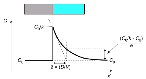
Fig.2 Steady state profile, showing how the solute boundary layer (δ) is defined.
Driving force for solidification
For a pure metal, at the fusion temperature, Tf, the Gibb’s free energy change for fusion, ΔGf, is zero, so that:
ΔGf = ΔHf - Tf ΔSf = 0
giving:
ΔHf = Tf ΔSf (1)
where ΔHf is the latent heat of fusion, and ΔSf is the entropy change upon melting.
For a temperature T, other than Tf:
ΔG = ΔH - T ΔS
ΔH and ΔS can be assumed to be constant for small changes is temperature, so for temperatures close to the fusion temperature:
ΔG ≈ ΔHf - Tf ΔSf (2)
Substituting (1) into (2) we get:
ΔG ≈ ΔHf - ΔSf ( Tf - T )
ΔG ≈ ΔSf ΔT
So the Gibb’s free energy change for solidification (also called the driving force) is proportional to the undercooling, ΔT, below the fusion temperature.
Derivation of the Scheil equation
Equating the amount of solute in the shaded areas gives:
( CL - C>S ) df = ( 1 - f ) dCL
Substituting for CS, using:
CS = k C0
where k is the partition coefficient gives:
CL ( 1- k ) df = ( 1 - f ) dCL
We then integrate, from zero to fS, the fraction solidified, and from C0 (since CL = C0 when fS = 0) to CL:
\[\int_0^{{f_S}} {\frac{{df}}{{\left( {1 - f} \right)}} = \int_{{C_0}}^{{C_{\rm{L}}}} {\frac{{d{C_{\rm{L}}}}}{{{C_{\rm{L}}}\left( {1 - k} \right)}}} } \]
\[ - \ln \left( {1 - {f_{\rm{s}}}} \right) = \frac{1}{{1 - k}}\ln \frac{{{C_{\rm{L}}}}}{{{C_0}}}\]
Taking exponentials of both sides, and rearranging gives:
CL = C0 ( 1 - fS )k-1
We are more interested in the concentration of the solid, so this is usually written as:
CS = k C0 ( 1 - fS )k-1
This is known as the Scheil equation.
Academic consultant: Noel Rutter (University of Cambridge)
Content development: Peter Marchment
Photography and video: Brian Barber and Carol Best
Web development:David Brook
This DoITPoMS TLP was funded by the UK Centre for Materials Education and the Department of Materials Science and Metallurgy, University of Cambridge
Additional support for the development of this TLP came from the Worshipful Company of Armourers and Brasiers'