Introduction To Anisotropy (all content)

Note: DoITPoMS Teaching and Learning Packages are intended to be used interactively at a computer! This print-friendly version of the TLP is provided for convenience, but does not display all the content of the TLP. For example, any video clips and answers to questions are missing. The formatting (page breaks, etc) of the printed version is unpredictable and highly dependent on your browser.

Contents

Main pages

Additional pages

Aims

On completion of this TLP you should:

• Understand the concept of anisotropy, and appreciate that the response (e.g. displacement) need not be parallel to the stimulus (e.g. force)
• Understand the nature of anisotropic behaviour in a range of properties, including electrical and thermal conductivity, diffusion, dielectric permittivity and refractive index, and be aware of a range of everyday examples
• Be familiar with the use of representation surfaces

Before you start

There are no specific prerequisites for this TLP, but you will find it useful to have a basic knowledge of crystal structures, as this will enable a better understanding of the structural origins of anisotropy. Take a look at the Crystallography TLP and the Atomic Scale Structure of Materials TLP.

Introduction

Some physical properties, such as the density or heat capacity of a material, have values independent of direction; they are scalar properties. However, in contrast, you will see that many properties vary with direction within a material. For example, thermal conductivity relates heat flow to temperature gradient, both of which need to be specified by direction as well as magnitude - they are vector quantities. Therefore thermal conductivity must be defined in relation to a direction in a crystal, and the magnitude of the thermal conductivity may be different in different directions.

A perfect crystal has long-range order in the arrangement of its atoms. A solid with no long-range order, such as a glass, is said to be amorphous. Macroscopically, every direction in an amorphous structure is equivalent to every other, due to the randomness of the long-range atomic arrangement. If a physical property relating two vectors were measured, it would not vary with orientation within the glass; i.e. an amorphous solid is isotropic. In contrast, crystalline materials are generally anisotropic, so the magnitude of many physical properties depends on direction in the crystal. For example, in an isotropic material, the heat flow will be in the same direction as the temperature gradient and the thermal conductivity is independent of direction. However, as will be demonstrated in this TLP, in an anisotropic material heat flow is no longer necessarily parallel to the temperature gradient, and as a result the thermal conductivity may be different in different directions.

The occurrence of anisotropy depends on the symmetry of the crystal structure. Cubic crystals are isotropic for many properties, including thermal and electrical conductivity, but crystals with lower symmetry (such as tetragonal or monoclinic) are anisotropic for those properties.

Many (but not all) physical properties can be described by mathematical quantities called tensors. A non-directional property, such as density or heat capacity, can be specified by a single number. This is a scalar, or zero rank tensor. Vector quantities, for which both magnitude and direction are required, such as temperature gradient, are first rank tensors. Properties relating two vectors, such as thermal conductivity, are second rank tensors. Third and higher rank tensor properties also exist, but will not be considered here, since the mathematical descriptions are more difficult.

Mechanical analogy of anisotropic response

A stimulus (such as a force or an electrical field) does not necessarily induce a response (such as a displacement or a current) parallel to it.

This can be demonstrated with a simple mechanical model, consisting of a mass supported by two springs.

Mechanical model: a mass supported by two springs

A force, F, applied at an angle θ, to the central mass acts as the stimulus. The response is the displacement, r, of the mass, at an angle φ.

Diagram showing applied force and resulting displacement

For second rank tensor properties in anisotropic materials, parallel responses occur along orthogonal directions known as the principal directions.

The following photographs show the response of the model under the application of various forces. (Click on an image to view a larger version.)

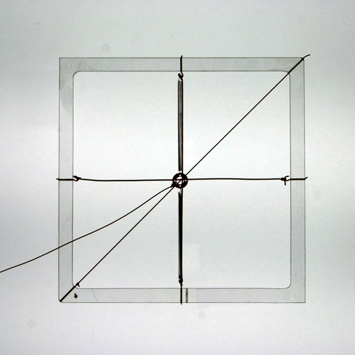
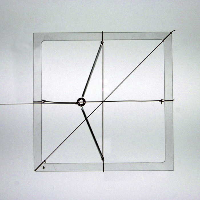
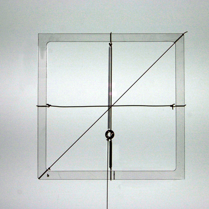
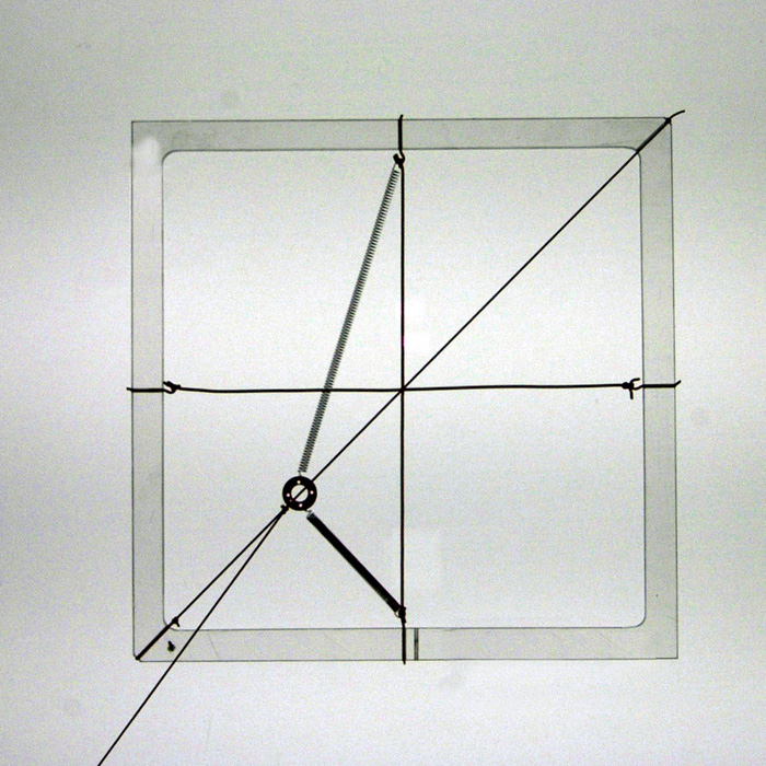
Note that the displacement of the mass is only parallel to the force when the force acts parallel or perpendicular to the springs. These are the directions of the principal axes.

Symmetry

As a rule, the symmetry present in crystalline materials (such as mirror planes and rotational axes) determines or restricts the orientation of the principal axes. In this model, there exist two orthogonal mirror planes perpendicular to the plane of the model, one parallel and the other perpendicular to the springs, and a third mirror plane exists in the plane of the model. The principal axes lie along the intersections of these mirror planes. Real crystals typically show more complicated symmetry, but the orientation of the principal axes is still determined by the main symmetry elements.

Anisotropic properties may be analysed by resolving onto these principal axes.

The symmetry elements of any physical property of a crystal must include the symmetry elements of the point group of the crystal (Neumann’s Principle). Thus crystals that, for example, display spontaneous polarization (see later section on anisotropic dielectric permittivity) can belong to only a few symmetry classes. It is worth noting that the absence of a centre of symmetry does not necessarily imply anisotropic second rank tensor properties, nor does the presence of a centre of symmetry rule out anisotropy in such properties.

Anisotropic thermal conductivity

When a temperature gradient is present in a material, heat will always flow from the hotter to the colder region to achieve thermal equilibrium. As mentioned in the introduction, thermal conductivity is the property that relates heat flow to the temperature gradient. In an isotropic material:

\[J = k{{dT} \over {dr}}\]

where J = heat flow, k = thermal conductivity, and dT/dr = temperature gradient.

Anisotropic thermal conductivity in quartz.

In quartz, perpendicular to the c-axis, the thermal conductivity is 6.5 Wm^-1K^-1. However, the thermal conductivity parallel to c is 11.3 Wm^-1K^-1.

The anisotropic thermal conductivity of quartz can easily be seen using a simple demonstration. Two sections cut from a quartz crystal, one perpendicular to the c-axis, and one parallel to it, are in turn mounted as shown in the diagram below. Pieces of plastic containing a heat sensitive liquid crystal are then glued to the top surfaces and the sections are heated from a point at their centre, using a soldering iron. As the quartz heats up, the heat sensitive film changes colour, which allows us to see how quickly the heat is conducted away from the centre. The colours indicate contours of constant temperature.

Diagram of experimental apparatus

When heating the section cut perpendicularly to the c-axis, the observed shape is a circle, showing that the thermal conductivity is the same in all directions in this plane. However, when using the section cut parallel to the c-axis, the shape seen is an ellipse, which shows that the thermal conductivity in this plane is direction-dependent.

Video of a section of quartz cut perpendicular to the c axis being heated from a point at its centre

Video of a section of quartz cut parallel to the c axis being heated from a point at its centre

Flow Properties

The heat flow does not have to be parallel to the thermal gradient. A result of this can be seen by considering one-dimensional conduction in a long rod and a thin plate, both made of the same anisotropic material, arranged so that the normal to the plate and the length of the rod are oriented in an arbitrary general direction.

Thin Plate

Here the geometry of the set-up constrains the temperature gradient to be perpendicular to the plate. Due to the anisotropic nature of the material, the heat flux, J, will be in the direction shown, say. However, the thermal conductivity perpendicular to the plate is defined as the component of the heat flux parallel to the temperature gradient, j_||, divided by the magnitude of that gradient. Thus:

\[{k_{||}} = {{{j_{||}}} \over {gradT}}\]

Rod

Now the heat must flow along the rod, and the temperature gradient will be in a different direction, as shown. Here the thermal resistivity is defined as the component of the temperature gradient parallel to the rod, gradT_||, divided by the magnitude of the heat flux. Thus:

\[{\rho _{||}} = {{grad{T_{||}}} \over J}\]

where ρ is the resistivity.

These definitions hold for any situation where the heat flux and the thermal gradient are not parallel in an anisotropic material, in isotropic materials they will be parallel. It is important to realise that in anisotropic materials

\[{\rho _{||}} \ne {\raise0.7ex\hbox{$1$} \!\mathord{\left/ {\vphantom {1 {{k_{||}}}}}\right.\kern 0.01em} \!\lower0.7ex\hbox{${{k_{||}}}$}}\]

except along the principal axes. Only in isotropic materials is the resistivity always the reciprocal of the conductivity, and vice versa.

Note: By using a large, thin plate and a long rod, the effects of the alterations in the directions of heat flow and temperature gradient close to the edges (of the plate) or ends (of the rod) - "edge effects" and "end effects" - affect only a very small proportion of the sample and can be ignored.

More broadly, anisotropic properties should be represented as tensors, for example thermal conductivity can be written:

\[{j_i} = {k_{ij}}{(gradT_j)}\]

and the thermal resistivity can be written:

\[{gradT_i} = {\rho_{ij}}{j_j}\]

where k_ij and ρ_ij are second rank tensors, see Tensors in Materials Science.

Derivation of the anisotropy ellipsoid

The variation of anisotropic properties such as conductivity can conveniently be illustrated by a "representation surface". In many cases this is an ellipsoid.

Suppose a three-dimensional temperature gradient, gradT, lies along a direction specified by direction cosines l, m and n>, where, for example, l is the cosine of the angle between the x-axis and the temperature gradient vector. Then the components of the temperature gradient parallel to the principal axes will be:

\[grad{T_x} = (gradT)l\qquad grad{T_y} = (gradT)m\qquad grad{T_z} = (gradT)n\]

The components of the heat flux are:

\[{j_x} = {k_1}(gradT)l\qquad {j_y} = {k_2}(gradT)m\qquad {j_z} = {k_3}(gradT)n\]

where k₁, k₂ and k₃ are the values of thermal conductivity along the principal axes, x, y and z, and are called the principal values.

Hence, resolving back along the direction of the temperature gradient, the heat flux is:

\[{j_{||}} = {j_x}l + {j_y}m + {j_z}n = ({k_1}{l^2} + {k_2}{m^2} + {k_3}{n^2})gradT\]

Thus the value of the thermal conductivity, k_lmn, defined by

\[{k_{lmn}} = {{{j_{||}}} \over {gradT}}\]

is related to the principal values and the directional cosines by:

\[k = {k_1}.{l^2} + {k_2}.{m^2} + {k_3}.{n^2}\]

\[l = {\raise0.7ex\hbox{$x$} \!\mathord{\left/ {\vphantom {x r}}\right.\kern 0.01em} \!\lower0.7ex\hbox{$r$}}\;\;\; m = {\raise0.7ex\hbox{$y$} \!\mathord{\left/ {\vphantom {y r}}\right.\kern 0.01em} \!\lower0.7ex\hbox{$r$}}\;\;\; n = {\raise0.7ex\hbox{$z$} \!\mathord{\left/ {\vphantom {z r}}\right.\kern 0.01em} \!\lower0.7ex\hbox{$r$}}\]

Substituting in our equation for k gives:

\[k = {{{k_1}{x^2}} \over {{r^2}}} + {{{k_2}{y^2}} \over {{r^2}}} + {{{k_3}{z^2}} \over {{r^2}}} = {1 \over {{r^2}}}({k_1}{x^2} + {k_2}{y^2} + {k_3}{z^2})\]

Setting

\[r = {\raise0.7ex\hbox{$1$} \!\mathord{\left/ {\vphantom {1 {\sqrt k }}}\right.\kern 0.01em} \!\lower0.7ex\hbox{${\sqrt k }$}}\]

then

\[{{k_1}{x^2}} + {{k_2}{y^2}} + {{k_3}{z^2}} = 1\]

If all the principal values are positive (as they must be for thermal conductivity), then this equation describes the surface of an ellipsoid. The general equation of an ellipsoid (with semi-axes a,b,c) is:

\[{{{x^2}} \over {{a^2}}} + {{{y^2}} \over {{b^2}}} + {{{z^2}} \over {{c^2}}} = 1\]

Thus for this representation ellipsoid, the semi-axes are:

\[{1 \over {\sqrt {{k_1}} }},{1 \over {\sqrt {{k_2}} }},{1 \over {\sqrt {{k_3}} }}\]

The radius of this ellipsoid in a general direction is equal to the value of \({1 \over {\sqrt {{k}} }}\)in that direction. Thus the value of k in a particular direction - the ratio of the component of the heat flow in that direction to the magnitude of the temperature gradient in that direction - can easily be calculated from the radius in that direction.

An equivalent representation surface exists for electrical conductivity, and a similar representation surface exists for refractive index - the optical indicatrix. Both of these are discussed later in this TLP.

Using the representation surface for thermal conductivity

As shown above, the representation surface for thermal conductivity is an ellipsoid with semi-axes \({1 \over {\sqrt {{k_1}} }}\), \({1 \over {\sqrt {{k_2}} }}\) and \({1 \over {\sqrt {{k_3}} }}\). The distance between the centre of the ellipsoid and a point, P, on its surface, is equal to \({1 \over {\sqrt {{k}} }}\) at this point.

As well as determing the conductivity, the representation surface can be used to relate the directions of heat flow and the temperature gradient. If the temperature gradient is applied radially from the centre of the ellipsoid, then the direction of resulting heat flow is perpendicular to the tangential plane constructed from the point at which the thermal gradient meets the surface of the ellipsoid.

In an isotropic material, the representation surface will be a sphere, and the heat flow will be in the same direction as the temperature gradient. However, in an anisotropic material, heat flow is no longer necessarily parallel to the temperature gradient.

We will now revisit the anisotropic thermal conductivity of quartz.

Because of the crystal symmetry of quartz, k₁ = k₂  k₃, and so the representation surface for the thermal conductivity of quartz is a uniaxial ellipsoid of revolution. Depending on the relative values of k₁ and k₃, this is a shape either like a rugby ball (k₃ < k₁) or a Smartie (k₃ > k₁).

Consider sections of the ellipsoid:

1. Perpendicular to the c-axis:

   Since k₁ = k₂, this section is a circle, and the direction of heat flow is parallel to the temperature gradient.

   

2. Perpendicular to the b-axis (i.e. parallel to the c-axis).

   Since k₁  k₃, this section is an ellipse, and the direction of heat flow is no longer parallel to the temperature gradient, except in the directions of the principal axes (which here correspond to the semi-axes of the ellipse).

   

The direction of the heat flux is always parallel to the normal to the tangential plane drawn at the point at which the direction of the temperature gradient intersects the representation ellipsoid. This is called the radius-normal property.

View proof of the radius-normal property.

Anisotropic electrical conductivity

The current density, J, is related to the electric field, E, by

J = σE

In an analogous way to thermal conductivity, the current density does not have to be parallel to the electric field. Three different examples of anisotropic electrical conductivity are described here. These show how the anisotropy is related to the crystal structure.

In metals, conductivity occurs by transport of delocalised electrons through the crystalline lattice, under the influence of an applied electric field. The conductivity is limited by the scattering of the electrons by imperfections in the periodicity of the structure (vibrations, impurities, etc). Because of the high symmetry in cubic metals, the overall drift velocity is parallel to the electric field, i.e. there is an isotropic response. However in hexagonally "close packed" metals, the nature of the symmetry in the crystalline array allows the conductivity to be anisotropic. For example in cadmium, it varies from 1.3 x 10⁷ Sm^-1 along the six-fold axis to 1.5 x 10⁷ Sm^-1 perpendicular to that axis.

Graphite consists of layered planes of carbon atoms with a structure as shown below. The layers are stacked above one another in a staggered fashion, the spacing between layers being about 2.3 times the distance between the adjacent carbon atoms in a layer.

The Hexagonal Structure of Graphite Planes

Here the hexagonal carbon rings provide the delocalised electrons, allowing easy conduction within the planes. Conduction is very much less perpendicular to the planes (around three orders of magnitude smaller) - this is highly anisotropic behaviour. The structure also creates anisotropy in other properties of graphite, such as thermal conductivity and thermal expansion.

This planar anisotropy is also seen in high temperature superconductors like BiSrCaCuO. The copper oxide "ab" planes provide superconducting pathways for electrons, but such pathways are not available perpendicular to the planes.

Anisotropic diffusion

The rate of diffusion of a specific atomic species is measured in terms of the coefficient of diffusion, D, which relates the flux of atoms (number crossing unit area in unit time) to the concentration gradient. In an isotropic material:

J = -D(gradc)

where J = flux (number per unit area per unit time) of an atomic species across a plane normal to the concentration gradient, gradc. The negative sign indicates that the flux is from high to low concentrations. For an isotropic material, such as an amorphous solid, the diffusion coefficient is independent of temperature.

Flux and concentration gradient are both vectors, so the coefficient of diffusion is a second rank tensor in an anisotropic material. The diffusion is anisotropic and can be described by three principal values of D, in the same way as thermal and electrical conductivity. (Note: we are not concerned here with the dependence of diffusion on temperature).

Example: Diffusion of Ni in Olivine, (Mg,Fe)₂SiO₄

Olivine is the name for a series of minerals between two end members, fayalite (Fe₂SiO₄) and forsterite (Mg₂SiO₄). The two minerals form a solid solution where the iron and magnesium atoms can be substituted for each other without significantly changing the crystal structure. Olivine has an orthorhombic structure. The lattice parameters depend on the precise composition, but a typical set of values is: a = 0.49 nm, b = 1.04 nm, c = 0.61 nm.

The principal values of D for diffusion of nickel atoms in olivine also depend on the precise composition of the olivine. One set of values for an unspecified composition at 1423 K (1150ºC) is:

D_x = 4.40 x 10^-18 m²s^-1
D_y = 3.35 x 10^-18 m²s^-1
D_z = 124.0 x 10^-18 m²s^-1

where the values correspond to the diffusion coefficients along the x, y and z crystallographic axes respectively. The exact values are unimportant for this discussion, but it is important to appreciate that diffusion occurs much faster parallel to the z-axis than in directions in the plane perpendicular to it. This happens because of the way in which the atoms are arranged in the crystal structure, a plan view of which is shown below (projected down the x-axis).

Note that x = 0, 25, 50 and 75 represent the x-coordinates of the atoms (as a percentage of the unit cell dimension a).

Crystal structure of olivine (click on image to view a larger version)

As you can see, there are chains of M²⁺ sites (where M²⁺ represents a metal ion, in this case either Mg or Fe) parallel to the z-axis. Diffusion occurs by Ni²⁺ substituting for M²⁺ along these chains, making diffusion in this direction much faster than in any other.

Rotatable model of the olivine structure

Fast ion conduction

When the structure of a solid material contains a large number of vacant sites (as a consequence of its composition), then it is likely to show high ionic mobility for some species of ion (sometimes an anion, sometimes a cation), even at modest temperatures. A high ionic mobility means that charge can be transferred very easily, and conductivities can approach those of aqueous electrolyte solutions or molten salts.

For a material to be a fast ion conductor, there should be:

• a high concentration of charge carriers
• a high concentration of vacant sites in the structure
• a low activation energy for ionic migration

There are a number of different types of fast ion conductors. The material may be either a cationic or an anionic conductor, depending on the charge of the mobile ion. The material may also have a fully ionic structure, or the mobile ions may be in a covalent host structure. The dimensionality of the mobility can also vary: the ions may move through channels (1D), within layers of a structure (2D), or throughout the whole structure (3D).

Examples of fast ion conductors

1D fast ion conductors: Tungsten Bronzes, M_xWO₃

In these materials, WO₃ tetrahedra or octahedra form a covalent network. Usually either M⁺ or M²⁺ (for example Na⁺ or Cu²⁺) are the mobile ions, and these move along channels in the structure. As a result, the conductivity is very high in this direction. An example of a tungsten bronze is shown below, projected along the z-axis, which is parallel to the channel direction.

Structure of tungsten bronze

2D fast ion conductor: Sodium beta-alumina, Na β-Al₂O₃

Sodium beta-alumina consists of blocks of γ-alumina (which has a spinel structure, the details of which need not be considered here) connected by a layer of bridging oxygen and sodium ions. Not all the Na⁺ sites are occupied, and conduction occurs by the movement of the ions within this layer.

Structure of sodium beta-alumina

Anisotropic dielectric permittivity

When an electric field, E, is applied to a dielectric solid, positive and negative charges are displaced in opposite directions within the solid, creating polarisation, P. This is defined as the net dipole moment per unit volume. (An electrical dipole is created by a small separation of equal and opposite charges.)

In an isotropic material, these vectors are related by:

P = (e - 1)e_oE

e_o is the permittivity of free space, and e is the relative dielectric permittivity (a scalar constant in this case). As with the other examples, in anisotropic materials this scalar has to be replaced by a tensor. Often the occurrence of highly anisotropic dielectric permittivity is associated with ferroelecticity (spontaneous polarisation reversible by an electric field) and pyroelecticity (temperature dependent generation of polarisation).

Example: barium titanate

The high temperature form of BaTiO₃ has the cubic perovskite structure with a primitive cubic lattice. At 150°C, a = 0.401 nm. In the temperature range 0ºC to 120ºC, BaTiO₃ is tetragonal. At 100°C it has a = b = 0.400 nm and c = 0.404 nm.

The tetragonal-cubic phase transition is highlighted in the following video. It shows a thin section of barium titanate viewed between crossed-polars, which is heated through the transition temperature, and then allowed to cool naturally. Initially, the sample is below the transition temperature, and since the domains of the anisotropic tetragonal phase exhibit birefringence, it is brightly coloured when viewed between crossed-polars. When the sample reaches the transition temperature, the isotropic cubic phase forms, which appears black. The heat source is then removed, so the sample cools down and again undergoes a phase transition to return to the anisotropic tetragonal phase.

Video of barium titanate phase transition

In the tetragonal form, the Ti ion is displaced by a small distance, from the centre of the surrounding octahedron of nearest neighbour oxygen ions, along the z-direction. A spontaneous polarisation along the z-axis is generated, but by symmetry there is no polarisation in the x-y plane. Note that the polarsation can be orientated forwards or backwards along the tetragonal axis. This polarisation is easily changed by applying an electric field parallel to the z-axis, but a field applied to the x-y plane has little effect on the polarisation. Consequently the dielectric permittivity is anisotropic.

The refractive index, n, is given by the square root of the relative dielectric permittivity, i.e. . The resulting optical effects are considered in the next section.

Optical anisotropy and the optical indicatrix

In transparent materials with anisotropic dielectric permittivity, important optical effects can be observed. Recall that a light wave may be considered in terms of oscillating transverse electric and magnetic fields. Here we concentrate on the effects of the electric field. When discussing optical properties it is important to remember that this field is in a direction lying in the wavefront. It is not necessarily perpendicular to the direction of propagation. The interaction between the electric field and the material is governed by the dielectric permittivity discussed in the previous section. A large value of the permittivity gives rise to a large refractive index, and consequently the wave travels relatively slowly. (The refractive index n is related to the velocity of light in the medium, v, and the velocity in a vacuum, c, by n = c/v.)

In an anisotropic material the refractive indices can again be illustrated by a representation surface - the optical indicatrix. For each (orthogonal) principal direction in the anisotropic material, there is an associated principal refractive index. The variation of the refractive index with the plane of the wavefront can be represented by an ellipsoid. The semi-axes of this optical indicatrix are directly proportional to the principal refractive indices.

Optically isotropic materials (e.g. cubic crystals) have one refractive index, with a spherical indicatrix.

Crystals with one 3, 4 or 6 fold axis of symmetry have a principal axis of the ellipsoid along this symmetry axis. These uniaxial crystals have an indicatrix which is an ellipsoid with a circular cross-section perpendicular to the major symmetry axis – an ellipsoid of revolution. They have two principal refractive indices and one optic axis (parallel to the symmetry axis and so perpendicular to the circular section).

In general, the electric field of a light wave experiences two permitted vibration directions, known as the fast and slow directions, both in the plane of the wavefront, and determined by the shape of the indicatrix. Consider a section passing through the origin of the indicatrix for a uniaxial crystal, and orientated parallel to the wavefronts, as shown by the dotted line in the left-hand figure below. The two permitted vibration directions are given by the major and minor axes of this section. The corresponding refractive indices are the lengths of these axes. The section will be elliptical unless the light is travelling along the optic axis so that the plane of the wavefront coincides with the circular section of the ellipsoid.

The observation of two refractive indices for a general orientation of the wavefront is known as birefringence. Related effects such as stress-induced birefringence and photoelasticity are discussed in the Photoelasticity TLP.

The ordinary vibration direction lies in the circular section of the indicatrix (i.e. perpendicular to the optic axis) with refractive index n_o. Light travelling along the optic axis experiences just this refractive index - the ordinary refractive index.

The extraordinary vibration direction lies in the plane of the wavefront and perpendicular to the ordinary vibration direction, and has refractive index n'_e. The value of n'_e is determined from the ordinary refractive index and the principal extraordinary refractive index n_e, as follows.

Consider a cross-section of the indicatrix (as shown in the diagram on the right above), containing the optic axis and the extraordinary vibration direction, taking the x direction to be horizontal and the y direction to be vertical with respect to the plane of the image. The equation for this ellipse will be:

\[{{{x^2}} \over {n_o^2}} + {{{y^2}} \over {n_e^2}} = 1\]

For the point P, x = n_e'cosθ, and y = n_e'sinθ. Therefore

\[{{{{(n{'_e}\cos \theta )}^2}} \over {n_o^2}} + {{{{(n{'_e}\sin \theta )}^2}} \over {n_e^2}} = 1\]

For a general extraordinary wave, the direction in which the light energy travels, the ray direction, is no longer perpendicular to the wavefront. For an explanation see, for example, the link to Optical Birefringence in Going further.

As a side note, the relative magnitudes of n_o and n_e determine whether a material is defined as optically positive or negative, the optical sign.

Example: calcite rhomb

The birefringence (defined as \(|{n_0} - {n_e}|\)) in calcite is so large that two images can easily be observed when viewing an object through a suitable crystal with the naked eye. One of which is due to the ordinary wave (with electric field vibrating parallel to the ordinary vibration direction) and the other is due to the extraordinary wave (with electric field vibrating parallel to the extraordinary vibration direction).

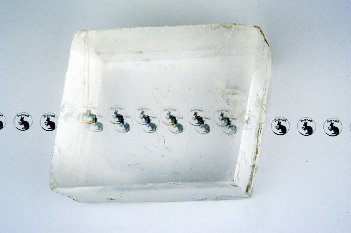
The DoITPoMS logo viewed through a calcite rhomb (click on image to view larger version)

In calcite, the planar carbonate groups all lie in planes normal to the three-fold axis - the optic axis. The groups are well separated in the direction of the axis. This makes the crystal less polarisable parallel to the axis, so the refractive index for vibrations parallel to the triad axis is smaller than for vibrations perpendicular to it (making the crystal optically negative: n_e < n_o).

Video of calcite structure

Liquid crystals

When most solids melt, they form an isotropic fluid, whose optical, electrical and magnetic properties do not depend on direction. However, when some materials melt, over a limited temperature range they form a fluid that exhibits anisotropic properties. These materials generally consist of organic molecules that have an elongated shape, with a rigid central region and flexible ends. The molecules in a liquid crystal do not necessarily exhibit any positional order, but they do possess a degree of orientational order.

The anisotropic behaviour of liquid crystals is caused by the elongated shape of the molecules. The physical properties of the molecules are different when measured parallel or perpendicular to their length, and residual alignment of the rods in the fluid leads to anisotropic bulk properties. This residual alignment occurs as a result of preferential packing arrangements, and also electrostatic interactions between molecules that are most favourable (lowest in energy) in aligned configurations.

There are three types of liquid crystal: nematic, smectic and cholesteric. In the liquid crystalline phase, the vector about which the molecules are preferentially oriented, n, is known as the "director". The long axes of the molecules will tend to align in this direction.

Three types of liquid crystal

In addition to the long range orientational order of nematic liquid crystals, smectic liquid crystals also have one dimensional long range positional order, the molecules being arranged into layers.

A cholesteric (or twisted nematic) liquid crystal is chiral: the molecules have left or right handedness. When the molecules align in layers, this causes the director orientation to rotate slightly between the layers, eventually bringing the molecules back into the original orientation. The distance required to achieve this is known as the pitch of the twisted nematic, as seen in the diagram above. The pitch is not equal to the distance marked x, because only 180º of rotation occurs over this length, so the molecules are aligned antiparallel to their starting orientation.

View examples of molecules that form liquid crystals.

When viewed between crossed polars, thin films (approximately 10μm thick) of liquid crystals exhibit schlieren textures, as seen in the micrograph below, which shows a nematic liquid crystalline polymer.

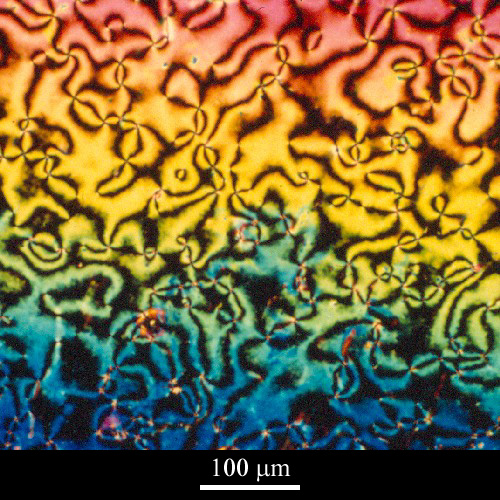
Micrograph of nematic liquid crystalline polymer, courtesy of Professor TW Clyne and the DoITPoMS Micrograph Library
(click on image to view larger version, or view full library record for the micrograph)

The black brushes are regions where the director is either parallel or perpendicular to the plane of polarisation of the incident radiation, and the points at which the brushes meet are known as disclinations.

If the temperature of a liquid crystal is raised, the constituent molecules have more energy, and are able to move and rotate more, so the liquid crystal becomes less ordered. As a result, the magnitude of the anisotropy of the bulk properties of the liquid crystal decreases, usually eventually resulting in an isotropic fluid.

Liquid crystals are used in many different applications, for example the displays on calculators, digital watches and mobile phones.

Summary

In some materials a property will be the same, irrespective of the direction in which it is measured, but this is not always the case. On completion of this TLP, you should now understand the concept of anisotropy, and be able to appreciate that a response can be non-parallel to the applied stimulus. Anisotropy in a range of properties has been discussed, including electrical and thermal conductivity, diffusion, dielectric permittivity, and optical properties. You should also now be familiar with the use of representation surfaces for a range of anisotropic properties, including the basis behind their mathematical description.

Anisotropic properties are exploited in many applications. In polarised-light microscopy, a quartz wedge can be used to determine birefringence and optical sign. Liquid crystals have electronic uses such as displays, and the liquid crystalline state has advantages in the processing of polymers (such as Kevlar). The anisotropic thermal conductivity in polymer thin films has use in microelectronic devices, for example, solid-state transducers.

Anisotropic properties described by higher than second rank tensors (not discussed here) can also have useful applications. Examples include:

• Piezoelectricity (relating an applied stress to the induced polarisation)
• The electro-optic effect (when a field causes a change in the dielectric impermeability)
• Elastic compliance and elastic stiffness (relating stress and strain)
• Piezo-optical effect (when a stress induces a change in refractive index)
• Electrostriction (strain arising from an electric field)

Non-tensor properties can also demonstrate anisotropy; for example, yield stress can vary with direction of applied stress.

Questions

1. Which of these properties of a crystal may be anisotropic?

   Yes	No	a	Density
   Yes	No	b	Young's modulus
   Yes	No	c	Surface energy
   Yes	No	d	Refractive index
   Yes	No	e	Electrical conductivity
   Yes	No	f	Thermal conductivity
   Yes	No	g	Heat capacity
   Yes	No	h	Melting point
   Yes	No	i	Coefficient of thermal expansion

2. Two similar transparent uniaxial crystals show the same (principal) extraordinary refractive index, n_e. However one is optically positive, and the other is optically negative. In which will the light travel faster along the optic axis?

3. Which of these could not induce anisotropy in an initially isotropic material?

   	a	Application of a stress
   	b	Application of an electric field
   	c	Application of a magnetic field
   	d	Application of a high temperature

4. Below 0°C a particular material has a crystal structure that gives rise to anisotropic thermal conductivity. At room temperature the thermal conductivity of a sample of this material is found to be isotropic. In what circumstances would the following hypotheses explain this observation?

   	a	The sample is polycrystalline
   	b	The sample has undergone a phase transition when brought up to room temperature
   	c	The principal values of thermal conductivity have changed with temperature

5. Which of these materials will show isotropy in its mechanical properties?

   	a	Wood
   	b	Carbon fibre reinforced polymer
   	c	Window glass
   	d	Extruded polyethylene

6. An olivine crystal has the following diffusion constants for Ni at a certain temperature:

   D_x = 6 x 10^-8 m²s^-1,
   D_y = 4 x 10^-18 m²s^-1
   D_z = 120 x 10^-18 m²s^-1.

   The unit cell dimensions are as follows:

   a = 0.5 nm
   b = 1.0 nm
   c = 0.6 nm

   By considering the representation surface, what will the diffusion constant be when the concentration gradient lies along the [101] direction?

7. A certain orthorhombic crystal has the following principal values of thermal conductivity:

   k_x = 6.25 Wm^-1K^-1
   k_y = 1.00 Wm^-1K^-1
   k_z = 1.75 Wm^-1K^-1

   (where the subscripts represent conductivity parallel to the x, y, and z axes respectively).

   The unit cell dimensions are: a = 0.8 nm, b = 0.6 nm, c = 1.0 nm.

   Calculate the thermal conductivity along the [111] direction.

8. Explain how anisotropy is involved in the operation of the following devices:
   

   1. a liquid crystal display
   2. a fuel cell that uses a sold state electrolyte
   3. a pyroelectric intruder alarm

9. Suggest ways of distinguishing between the answers to Question 4.

Going further

Books

• A. Putnis, Introduction to Mineral Sciences, CUP, 1992 (specifically Chapter 2, "Anisotropy and physical properties").
• R.E. Newnham, Structure-Property Relations Relations (Crystal chemistry of non-metallic materials), Springer-Verlag, 1975
• D.R. Lovett, Tensor Properties of Crystals, IOP, 1999
• P.J. Collings and M. Hird, Introduction to Liquid Crystals: Chemistry and Physics, Taylor & Francis, 1997

More advanced and detailed books:

• C. Kittel, Introduction to Solid State Physics, 7th Edition 1995
• J.F. Nye, Physical Properties of Crystals: Their Representation by Tensors and Matrices, Oxford, 2nd Edition 1985
• E. Hecht, Optics, Addison-Wesley, 4th Edition 2001

Websites

• Polymers and Liquid Crystals
  An award-winnning website based at Case Western Reserve University in the USA, with a Virtual Textbook and Virtual Laboratory.
• Introduction to Photoelasticity
  A TLP covering many features of birefringence under polarised light.
• Theoretical methods for Mineral Sciences research
  Summary of phase transitions and formation of domains in perovskites.
• Optical Birefringence
  This comprehensive introduction to optical birefringence is part of the excellent award-winning Molecular Expressions website based at Florida State University in the USA.
• Birefringence in calcite crystals
  Also part of the Molecular Expressions website, this is an interactive Java tutorial.

For some light relief, take a look at:

• The Optical Indicatrix - And Why I Love It So Much

Tensors

Tensor analysis can be used to describe this situation. Consider an anisotropic material with principal axes 1, 2 and 3. For sake of example, a temperature gradient, gradT, is applied in an arbitrary direction perpendicular to the 3-axis, non-parallel to the principal axes 1 and 2. The resulting heat flow, J, will not be parallel to the temperature gradient. The components of these vectors parallel to the principal axes are as shown in the diagram below.

As mentioned before, J = k(gradT). Using tensor notation to describe the above situation,

J₁ = k₁₁(gradT₁), J₂ = k₂₂(gradT₂), and J₃ = 0

In general,

J_i = k_ij(gradT_j)

where the suffices i and j represent the relevant axes. This equation summarises the following matrix equation:

Here J_i and gradT_j are first rank tensors (one suffix) and k_ij is second rank (two suffices). Since 1, 2 and 3 are the principal axes then the k_ij tensor is a diagonal matrix - all values are zero unless i = j. If an arbitrary set of axes is chosen, then it will be a general matrix.

Other second rank tensors, which relate first rank tensors, include:

• Electrical conductivity, relating current density to electric field
• Permittivity, relating dielectric displacement to electric field
• Permeability, relating magnetic induction to magnetic field

Thermal expansion is also a second rank tensor, but it relates strain (a second rank tensor) to temperature change (a scalar - zero rank).

Radius-normal property of the representation ellipsoid

As previously described, the heat flux, J, in an anisotropic material is related to the temperature gradient, gradT, by:

J = k(gradT)

The components of the temperature gradient parallel to the principal axes (x, y and z) will be:

\[grad{T_x} = (gradT)l grad{T_y} = (gradT)m grad{T_z} = (gradT)n\]

where l, m and n are the direction cosines specifying the direction of gradT, and for example, l is the cosine of the angle between the x-axis and the thermal gradient vector.

Therefore, the components of the heat flow are:

\[{j_x} = {k_1}(gradT)l\;\;\; {j_y} = {k_2}(gradT)m \;\;\; {j_z} = {k_3}(gradT)n\]

where k₁, k₂ and k₃ are the values of thermal conductivity along the principal axes, x, y and z, and are called the principal values.

The direction cosines of J> are therefore proportional to k₁l, k₂n, n₃n.

We have already shown that the equation for the representation ellipsoid is

\[{k_1}.{x^2} + {k_2}.{y^2} + {k_3}.{z^2} = 1\]

Suppose P is a point on the surface of the ellipsoid such that OP is parallel to the temperature gradient. The coordinates of P are therefore rl, rm, rn), where r is the distance OP.

\[r^2 = {k_1}{x^2} + {k_2}{y^2} + {k_3}{z^2}\]

The components of the gradient at (x₁ y₁z₁) are obtained by partial differentiation of this equation, which gives components in the directions of the x, y, and z axes of:

\[2r{{{\rm{d}}r} \over {{\rm{d}}x}} = 2{k_1}{x_1}\;\;\;2r{{{\rm{d}}r} \over {{\rm{d}}x}} = 2{k_2}{y_1}\;\;\;2r{{{\rm{d}}r} \over {{\rm{d}}x}} = 2{k_3}{z_1}\]

The components are therefore equal to

\[\left( {{{{k_1}{x_1}} \over r} , {{{k_2}{y_1}} \over r} , {{{k_3}{z_1}} \over r}} \right)\]

But since

x₁ = rl, y₁ = rm, z₁ = rn

the normal at P has direction cosines proportional to k₁l, k₂m, k₃n. Hence the normal at P is parallel to the heat flux.

Examples of molecules which form liquid crystals

4-methoxylbenzylidene-4'-butylaniline (MBBA) transforms from crystalline to nematic liquid crystal at 20ºC, and from nematic to an isotropic liquid at 74ºC

This very similar molecule forms a chiral nematic (cholesteric) liquid crystal. The chiral centre is marked with a *.

4-cyanobenzylidene-4'-n-octyloxyanaline (CBOOA) forms a smectic liquid crystal below 83ºC and a nematic liquid crystal between 83ºC and 109ºC.

Academic consultant: John Leake (University of Cambridge)
Content development: Chris Shortall and Jessica Gwynne
Photography and video: Brian Barber and Carol Best
Technical support: Helen Hignell
Web development: Dave Hudson

This TLP was prepared when DoITPoMS was funded by the Higher Education Funding Council for England (HEFCE) and the Department for Employment and Learning (DEL) under the Fund for the Development of Teaching and Learning (FDTL).