Coating Mechanics (all content)
Note: DoITPoMS Teaching and Learning Packages are intended to be used interactively at a computer! This print-friendly version of the TLP is provided for convenience, but does not display all the content of the TLP. For example, any video clips and answers to questions are missing. The formatting (page breaks, etc) of the printed version is unpredictable and highly dependent on your browser.
Contents
Main pages
Additional pages
Aims
On completion of this tutorial you should:
- Appreciate the meaning of a misfit strain between the stress-free (in-plane) dimensions of two layers
- Understand how misfit strains can arise and how they give rise to stresses and strains in the layers, depending on their elastic properties and thicknesses
- See how the general case is simplified when one of the layers (a coating) is much thinner than the other (a substrate) and understand the Stoney equation
- Be able to predict the curvature that tends to arise in such systems
- Be able to predict whether debonding is likely to occur, given the value of the interfacial fracture energy
Before you start
It may be helpful to study the Beam Bending TLP before you start, particularly the page covering Bending Moments and Beam Curvatures.
Introduction
This TLP covers some basic mechanics of multi-layered systems. It relates primarily to a 2-layer system, such as a coating on a substrate, although it should be fairly clear how the concepts involved can be extended to multi-layer systems. The treatments presented are for the general case, although the behaviour expected for the special case of one layer being much thinner than the other (eg a thin coating on a massive substrate) is also described.
The TLP is focused on the distributions of (in-plane) stress and strain that can arise within the two constituents under various imposed conditions. These could include applying well-defined external forces, such as an in-plane load or a bending moment. In those cases, the response of the system (in-plane extensions or out-of-plane curvatures) can be obtained from well-known expressions related to the mechanics of composites or of beam bending. However, in layered systems, such as coatings on substrates, the imposed conditions are often more complex than this. For example, heating or cooling of the system will lead to differential thermal expansion or contraction, generating a misfit strain - that’s to say, a difference between the stress-free (in-plane) dimensions of the two constituents. Misfit strains, which can also arise in other ways (such as plastic deformation of one of the layers), are important in the mechanics of layered systems. They can give rise to relatively complex through-thickness distributions of stress and strain, and also to both in-plane length changes and out-of-plane curvature.
It may also be noted that misfit strains can arise simultaneously in more than one in-plane direction. In fact, it is common for a given misfit strain to be generated in all in-plane directions - this would normally be the case for differential thermal contraction, assuming in-plane isotropy of the thermal expansion coefficients. As a consequence of Poisson effects, this effectively raises the in-plane stiffness (ratio of stress to strain in any given direction), which can be handled by simply using a biaxial stiffness in place of the conventional one.
Misfit strains
The Concept of a Misfit Strain
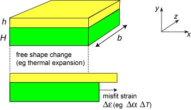
An important concept in layered (and other) systems is that of a misfit strain - ie a difference between the stress-free dimensions of two or more constituents that are bonded together. It is relevant to composite materials and also to macroscopic systems such as two or more components that are bolted or welded together in some way. In general, this strain is a tensor, with principal axes and three principal values. For a layered system, however, the focus is on a single (in-plane) direction, so that the strain can be treated as a scalar.
A simple type of misfit strain is that arising from differential thermal expansion (in a 2-layer system). In general, one layer will expand more during heating than the other (in the direction concerned). If the two layers were not bonded together, then they would behave as shown in the figure below. The misfit strain (in the x-direction) is given by the product of the difference in expansivity between the two constituents and the temperature change. It is often written as Δε. The fact that the two layers are actually bonded together leads to creation of internal stresses and strains, and to changes in the shape of the system - see the next page.
Sources of Misfit Strains
What are effectively misfit strains can arise in a number of ways. One of the simplest is differential thermal contraction, but anything that creates a difference between the (in-plane) stress-free dimensions of a substrate and a coating (or a surface layer of a substrate) has a similar effect. These include phase changes, plastic deformation, creep etc, as well as phenomena, such as atomic bombardment, that can create stresses during formation of a coating.
- \( \Delta \alpha \Delta T \)
- Phase transformations (eg solidification, resin curing, martensitic transformations)
- Plastic deformation (eg shot peening)
- Creep
- (Such deformation can also modify existing Δε values.)
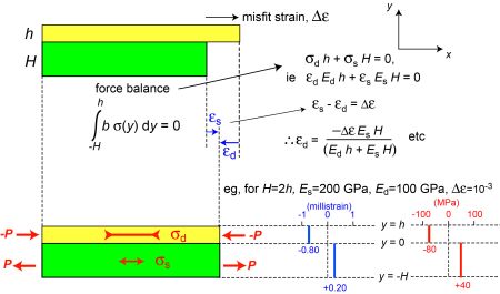
Force and moment balances
Force Balance
The fact that the two layers are in fact bonded together must now be taken into account. Assuming first that the layers remain flat, there is clearly a requirement that both must end up with the same length (in the x-direction). This will require a tensile stress to be created in one layer (the one that is initially shorter) and a compressive stress in the other. The forces acting in each layer (in the x-direction) must add up to the externally applied force (ie a force balance must apply). Since there is no applied force in the case we are currently considering, the forces in the two layers must sum to zero. In addition, the misfit strain must be partitioned in some way between the two layers. There are thus two simultaneous equations, allowing the solution to be found. This is illustrated in the figure below. (The subscripts d and s represent “deposit” and “substrate” - ie the upper and lower layers.)
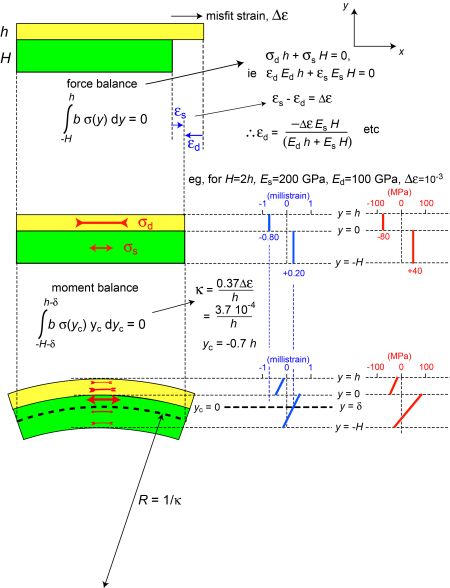
Moment Balance
The force balance is relatively straightforward, but the situation depicted in the figure above does not represent complete static equilibrium. This is because the forces being exerted by the stresses acting in the two layers produce a bending moment that tends to create curvature in the x-y plane - for the case shown, the top surface would become convex. The distributions of stress and strain must therefore change, creating an internal balancing moment (and also creating curvature), while maintaining a force balance.
Using the moment balance to find the curvature (and the associated stress and strain distributions) is slightly more complex than applying the force balance. Derivation of the expression for the curvature is shown here. The outcome is:
\[ \kappa = \frac{{6{E_d}{E_s}\left( {{h} + {H}} \right){h}{H}\Delta \varepsilon }}{{{E_d}^2{h}^4 + 4{E_d}{E_s}{h}^3{H} + 6{E_d}{E_s}{h}^2{H}^2 + 4{E_d}{E_s}{h}{H}^3 + {E_s}^2{H}^4}} \]
It’s important to recognize that the curvature of a beam is equal to the through-thickness gradient of the associated (in-plane) strain distribution. The other key concept here is that of the neutral axis of the beam. This is the location - strictly, it’s a plane (in 3-D), rather than an axis - where no (in-plane) strains arise from the bending (adoption of curvature). Its location, for a 2-layer system, is derived here. The result is:
\[ \delta = \frac{{\left( {{h^2}{E_d} - {H^2}{E_s}} \right)}}{{2\left( {h{E_d} + H{E_s}} \right)}} \]
Using these equations, the final outcome (of imposing a misfit strain) can be obtained. This is illustrated in the figure below. It should be noted that adoption of curvature does NOT lead to zero strain at the neutral axis, but rather to NO CHANGE there - ie it remains at the value resulting from the force balance. (If we simply applied an external bending moment, rather than an internal misfit strain, then there would be no strain at the neutral axis.)
The biaxial modulus
Biaxial Stress States
So far, attention has been concentrated on a single (in-plane) direction. For conventional (in-plane) uniaxial loading of a bilayer sample, or for applying a bending moment to it, this is appropriate. It’s also possible to generate a misfit strain in a single (in-plane) direction. However, while this is possible, it’s actually rather unusual. More commonly, the same misfit strain is generated simultaneously in all in-plane directions, a state that can be represented by creating the strain in two arbitrary (in-plane) directions that are normal to each other. This will lead to an Equal Biaxial stress state (since all in-plane directions are clearly equivalent and the through-thickness stress, σy, is often taken to be zero - there is no normal stress at a free surface). Differential thermal contraction would normally have this effect. It’s also possible to create an Unequal Biaxial stress state. This would arise, for example, during differential thermal contraction with one or both of the layers exhibiting in-plane anisotropy in thermal expansivity, so that the misfit strain would be different in different in-plane directions. (Also, anisotropy in stiffness would lead to different stresses in different in-plane directions, even if the misfit strains were equal.) It is, however, common to at least assume that all in-plane directions are equivalent, in terms of both properties and misfit strains.
Poisson Effects
The main reason why the case of an equal biaxial misfit strain differs from that of a uniaxial one is related to Poisson effects. The strains arising in the selected in-plane direction (the x-direction) will be accompanied by Poisson strains in the other two (principal) directions. That in the through-thickness (y) direction is often of little consequence, but in the other in-plane (z) direction, it will need to be added to the outcome of the effects arising in that direction (from the misfit strain in that direction). The upshot of this is actually rather simple. By symmetry, the two in-plane stresses (and strains) must be equal - ie σx = σz. For isotropic elastic properties and no through-thickness stress (σy = 0), the strain in the x-direction can be written in terms of the three principal stresses:
\[{ε_x}E = {\sigma _x} - \nu \left( {{\sigma _y} + {\sigma _z}} \right) = {\sigma _x}\left( {1 - v} \right)\]
where ν is the Poisson ratio. The ratio of stress to strain in the x-direction (and all in-plane directions) can therefore be expressed
\[ \frac {{\sigma _x}}{\epsilon_x} = \frac {{E}}{ \left(1 - \nu \right)} = E{^{'}} \]
This modified form of the Young’s modulus, E’ (often termed the Biaxial Modulus), is applicable in expressions referring to substrate/coating systems having an equal biaxial stress state. The effective stiffness (stress/strain ratio) has been raised by this Poisson effect. This higher value should be used in place of E throughout the formulations in the preceding pages (when the misfit strain is generated in all in-plane directions).
The Stoney Equation - the Thin Coating Limit
Origin of the Stoney Equation
The Stoney equation is still in widespread use. It relates the curvature of a substrate with a thin coating to the stress level within the coating (for an equal biaxial case). It was proposed in 1909 - a long time before the relationship described in earlier pages (for the general case in which the coating thickness is not negligible compared to that of the substrate) was established. However, it is easy to show that the Stoney equation can be derived from that relationship, by imposing the h << H condition, which allows all of the denominator terms except the last one to be discarded and (h + H) = H to be assumed, so that
\[ \kappa = \frac{{6{E{^{'}_\rm{d}}}h \Delta \epsilon }}{{{E{^{'}_\rm{s}}}{H^2}}} \]
with the biaxial moduli now being used. Furthermore, the h << H condition allows the assumption to be made that all of the misfit strain is accommodated in the coating (deposit), so only the coating is under stress. In addition, the Stoney equation is based on an equal biaxial stress state, so that the biaxial versions of these Young’s moduli should be used and the misfit strain can be expressed as
\[ \Delta \epsilon = \frac{{−\sigma_d}}{E{^{'}_\rm{d}}} \]
recognizing that, with the convention we are using for \( \Delta \epsilon \), a positive value will generate a negative value for \( \sigma_\rm{d} \) (ie a compressive stress). Substitution of this then leads to the Stoney equation:
\[ \kappa = \frac{{−6{E{^{'}_\rm{d}}}h \sigma_\rm{d} }}{{{E{^{'}_\rm{s}}}{H^2}{E{^{'}_\rm{d}}}}} = \frac{{−6h \sigma_\rm{d} }}{{{E{^{'}_\rm{s}}}{H^2}}} \;\;\; ∴\; {\sigma_\rm{d}} = \frac{− {E{_\rm{s}}{H^2}}}{6h \left( {1 − {\nu_\rm{s}}} \right)}\kappa \]
(The minus sign is not always included, but the curvature should have a sign and, using the convention that a convex upper surface corresponds to positive curvature, this implies a negative deposit stress.) This equation allows a coating stress to be obtained from a (measured) curvature. Only \( E \) and \( \nu \) values for the substrate are needed - this is convenient, since they are often known (whereas those of the coating may not be). A single stress value is obtained - if the coating is thin, then any through-thickness variation in its value is likely to be small. It is really the misfit strain that is the more fundamental measure of the characteristics of the system, but a stress value is often regarded as more easily interpreted.
Approach to Stoney Conditions
The Stoney equation is easy to use and, indeed, is widely used. However, it does have the limitation of being accurate only in a regime in which the curvatures tend to be relatively small. In some applications – such as with semiconductor wafers – surfaces are very smooth, so that highly accurate optical methods of curvature measurement are feasible and this is not such a problem. However, when curvatures are high (or need to be high for reliable measurement), the Stoney equation should not be used. The simulation below allows exploration of the conditions under which the Stoney equation gives a good or poor approximation to the actual behaviour. It should be noted that, while the stresses are scale-independent, the curvatures are not - changing the substrate thickness thus affects the plots on the left, but not those on the right.
Spallation (Interfacial Debonding)
Driving Force for Spallation
The presence of residual stresses in a substrate/coating system constitutes a driving force for debonding (spallation), since such stresses will almost certainly be at least partially relaxed when this occurs, releasing stored elastic strain energy. The key process is that of propagation of a crack along the interface, driven by the associated release of this stored energy. This propagation is illustrated below, for a (Stoney) case in which there is just a single (uniform) stress in the coating.
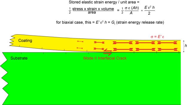
It can be seen that propagation of this interfacial crack will be energetically favoured if the driving force (strain energy release rate) is equal to or greater than the (mode II - ie shearing mode) fracture energy of the interface, Gic:
\[ E{^{'}}_d \epsilon _d^2 h \left( = \frac{{\sigma _d^2}h}{{E_d^{’}}} \right)\geq G_{\rm{ic}} \]
This takes no account of any barrier to initiation of the crack. In many cases, however, there are likely to be relatively large defects present in the interface, so the above condition may well lead to spallation. It certainly means that the coating is (thermodynamically) unstable. Immediate implications are (unsurprisingly) that high stresses and brittle interfaces (low Gic) make debonding more likely. Also clear (and widely observed) is that thicker coatings are more likely to debond than thinner ones.
Debonding for non-Stoney Cases
The same concept can be applied to more general cases - ie when the h<<H condition does not apply. Debonding will still tend to allow a reduction in the stored elastic strain energy, constituting a driving force for spallation. However, since there is now a distribution of stress (and strain) in the through-thickness (y) direction, an integration is needed to evaluate the driving force
\[ {G_i} = \mathop \smallint \limits_{ - H}^h \frac{{\sigma {{\left( y \right)}^2}}}{{E^{’}\left( y \right)}}{\rm{d}}y \]
This is based on the assumption that these stresses become totally relaxed during debonding. This might be the case - for example, the sets of stresses and strains that have been predicted to arise from imposition of a uniform misfit strain would completely disappear if the coating could debond. In practice, however, the stress distribution within the system may be more complex than this. For example, it’s common for stresses to be created in a coating during its formation. As such a coating gets thicker, balancing of forces and moments takes place progressively, so that conditions change and the final stress distribution is not one corresponding to imposition of a uniform misfit strain. In such cases, debonding may leave some residual stresses (and residual curvature of the coating and possibly of the substrate). The net driving force may then be written
\[ {G_i} = \mathop \smallint \limits_{ - H}^h \frac{{\sigma {{\left( y \right)}^2}}}{{E^{’}\left( y \right)}}{\rm{d}}y - \mathop \smallint \limits_{ - H}^h \frac{{{\sigma _r}{{\left( y \right)}^2}}}{{E'\left( y \right)}}{\rm{d}}y \]
where σr(y) is the residual stress distribution after debonding.
Debonding of coatings is, of course, commonly observed, since virtually all coatings contain at least some stresses and the associated strain energy can rise above the critical level - for example, as a result of temperature changes, thickening (eg oxide growth), stiffening (eg due to sintering), applied forces or bending moments etc. Also, the toughness (fracture energy) of the interface (Gic) may fall with time - eg due to chemical attack etc. The video clips below give some examples of how coating spallation can be observed and analysed.
Spontaneous Debonding. This video shows a set of coated samples (zirconia on alumina substrates) being withdrawn from a furnace and cooled by gas jets. The cooling creates differential thermal contraction stresses and, once these have become sufficiently large, coatings can spontaneously debond. Such an event can be seen at the end of this short video.
In Situ Curvature Measurement. This video, which has a commentary, explains how, provided the substrate is relatively thin, the deposition of a coating (in this case by thermal spraying of ceramics onto metal substrates) generates curvature, which can be monitored as the coating thickness increases. In conjunction with a numerical model, this can be used to infer the residual stress levels in coatings produced under a range of conditions.
Debonding during Cooling of Thin Substrate with Coatings. This video, which has a commentary, explains how stored residual stresses provide a driving force for debonding (spallation). It is also explained how estimates can be made of the interfacial toughness (fracture energy) from observations of debonding during cooling.
Debonding under Applied Load of Coatings with Residual Stresses. This video, which has a commentary, goes briefly through the 4-point bend delamination test for coatings that already contain stored residual stresses. It is shown how this can be used to measure the interfacial fracture energy.
Summary
A coating on a planar substrate is an important special case of a composite system. Attention is concentrated here on the mechanical (stress-related) effects that commonly arise, with the possibility of stresses (in-plane only) and strains within both constituents being generated in a variety of ways. In the treatment presented here, edge effects are ignored, which simplifies matters, but considerable attention is paid to the way in which the system may become curved, and to the relationship between the curvature and the internal stresses and strains.
Two main cases are considered, depending on whether it is possible for the assumption to be made that the coating is very much thinner than the substrate. If this is the case, then certain assumptions can be made and some relatively simple equations can be used to describe the behaviour. On the other hand, it is emphasized that there are many practical cases for which this condition cannot be assumed, although (slightly more complex) analytical treatments can then be employed and these are described here in some detail.
It is also worth noting that a further distinction can be drawn, depending on whether the stress state within the coating (and substrate) comprises a uniaxial (in-plane) stress or an equal biaxial set of (in-plane) stresses, with the latter being much more common. In this case, it is explained that the ratio of stress to strain in any given (in-plane) direction is given by the biaxial modulus, rather than the Young’s modulus (for a uniaxial stress state).
Finally, a brief outline is presented of how the stored elastic strain energy associated with the presence of stresses in a coating (and substrate) constitutes a driving force for spallation (interfacial crack propagation). A simple criterion is presented for advance of such a crack and some examples are given of how this can be utilized in some practical cases.
Questions
Quick questions
You should be able to answer these questions without too much difficulty after studying this TLP. If not, then you should go through it again!
-
What is meant by a "misfit strain"?
-
Why does curvature tend to arise in a coating-substrate system, as a result of the stresses in each constituent caused by imposing a force balance?
-
Which of these conditions is sufficient to ensure that the Stoney equation is a good approximation for the relationship between coating stress and curvature?
-
What is meant by the "Biaxial Modulus" of a coating (or a substrate) and why is it greater than the conventional (Young's modulus)?
Deeper questions
The following questions require some thought and reaching the answer may require you to think beyond the contents of this TLP.
-
How is the neutral axis (strictly, the neutral plane) of a beam defined?
-
Which of these definitions of the curvature of a beam is correct?
-
Which of these statements regarding debonding (spallation) of coatings is incorrect?
Going further
Books
There are not really any books that specifically cover all of the material in this TLP, although there are, of course, books that treat various aspects of coatings, and of surface engineering more generally. The three below respectively present a review of developments since the original Stoney equation, modelling of progressive deposition of a coating onto a thin substrate and the anisotropy that arises with thin films on (cubic) single crystal substrates.
MR Begley & JW Hutchinson, The Mechanics and Reliability of Films, Multi-layers and Coatings, CUP (2017) ISBN: 9781107131866.
J Mencik, Mechanics of Components with Treated or Coated Surfaces, Springer (2010) ISBN-13: 978-9048146116.
L. B. Freund & S. Suresh, Thin Film Materials: Stress, Defect Formation and Surface Evolution, CUP (2004) ISBN-1139449826
Other resources
There are many journal papers that cover the issue of stresses and strains in surface coatings and also the broader topics of how they can provide various kinds of protection, including thermal, environmental and tribological. The two below respectively present a review of developments since the original Stoney equation and an outline of how progressive deposition of a coating onto a thin substrate can be treated.
GCAM Janssen, MM Abdalla, F van Keulen, BR Pujada & B van Venrooy, Celebrating the 100th Anniversary of the Stoney Equation for Film Stress: Developments from Polycrystalline Steel Strips to Single Crystal Silicon Wafers, Thin Solid Films, 517 (2009) p.1858-1867, https://doi.org/10.1016/j.tsf.2008.07.014
YC Tsui & TW Clyne, An Analytical Model for Predicting Residual Stresses in Progressively Deposited Coatings .1. Planar Geometry, Thin Solid Films, 306 (1997) p.23-33, https://doi.org/10.1016/S0040-6090(97)00199-5
KM Knowles, The Biaxial Moduli of Cubic Materials Subjected to an Equi-biaxial Elastic Strain, J. of Elasticity, 124 (2016) p.1-25, https://doi.org/10.1007/s10659-015-9558-x
Relation between Curvature and Misfit Strain
Referring to the figure in the Force Balance section, the forces P and –P generate a moment, given by
\[M = P\left( {\frac{{h + H}}{2}} \right)\]
where h and H are deposit and substrate thicknesses respectively. Since the curvature, κ, (through-thickness strain gradient) is given by the ratio of moment, M, to beam stiffness, Σ
\[\kappa = \frac{M}{{\rm{\Sigma }}}\]
P can be expressed as
\[P = \frac{{2\kappa {\rm{\Sigma }}}}{{h + H}} (i)\]
The beam stiffness is given by
\[ {\rm{\Sigma }} = b\mathop \smallint \limits_{ - H - \delta }^{h - \delta } E\left( {{y_c}} \right)y_c^2 d{y_c} = b{E_\rm{d}}h\left( {\frac{{{h^2}}}{3} - h\delta + {\delta ^2}} \right) + b{E_\rm{s}}H\left( {\frac{{{H^2}}}{3} + H\delta + {\delta ^2}} \right) (ii) \]
where δ (the distance between the neutral axis (yc = 0) and the interface (y = 0)) is given by
\[ \delta = \frac{{\left( {{h^2}{E_\rm{d}} - {H^2}{E_\rm{s}}} \right)}}{{2\left( {h{E_\rm{d}} + H{E_\rm{s}}} \right)}} (iii)\]
The magnitude of P is found by expressing the misfit strain as the difference between the strains resulting from application of the P forces (ie by writing a strain balance):
\[\Delta ε = {ε_\rm{s}} - {ε_\rm{d}} = \frac{P}{{Hb{E_\rm{s}}}} + \frac{P}{{hb{E_\rm{d}}}}\]
\[ \frac{P}{b} = Δ ε \left(\frac{{ {h{E_\rm{d}}H{E_\rm{s}}} }}{{h{E_\rm{d}} + H{E_\rm{s}}}}\right) (iv) \]
Combination of this with Eqns.(i)-(iii) gives a general expression for the curvature, κ, arising from imposition of a uniform misfit strain, \(\Delta ε \)
\[ \kappa = \frac{{6{E_\rm{d}}{E_\rm{s}}\left( {h + H} \right)hH Δ ε }}{{{E_\rm{d}}^2{h^4} + 4{E_\rm{d}}{E_\rm{s}}{h^3}H + 6{E_\rm{d}}{E_\rm{s}}{h^2}{H^2} + 4{E_\rm{d}}{E_\rm{s}}h{H^3} + {E_\rm{s}}^2{H^4}}} (v)\]
The stress at the interface (y = 0), and at the free surfaces (y = h or -H), can be written in terms of the base level in each constituent (arising from the force balance) and the change due to the stress gradient (= curvature × stiffness):
\[ \left. \sigma{_d} \right|_{y=h} = \frac{{-P}} {b h} + {E_\rm{d}}\kappa \left(h - \delta \right) \]
\[\left. \sigma{_d} \right|_{y=0} = \frac{{-P}} {b h} − {E_\rm{d}}\kappa{\delta} \]
\[ \left. \sigma{_s} \right|_{y=-H} = \frac{{P}} {b h} − {E_\rm{s}}\kappa \left(H + \delta \right) \]
\[ \left. \sigma{_s} \right|_{y=0} = \frac{{P}} {b h} − {E_\rm{s}}\kappa{\delta} \]
Since the gradient is linear in each constituent, this gives the complete stress profile.
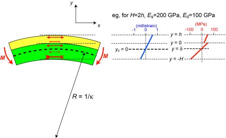
Location of the Neutral Axis for a Bi-layer System
The figure below shows how the application of a bending moment, M, creates curvature, which is equal to the through-thickness strain gradient. Its magnitude depends on the applied moment and the beam stiffness of the sample. An example strain gradient is shown in the figure. Using the stiffness values shown, corresponding stresses can be found and these are also plotted.
The force balance
\[ b\mathop \smallint \limits_{ - H}^h \sigma (y) dy = 0 \]
can be divided into contributions from the two constituents and expressed in terms of the strain
\[ b\mathop \smallint \limits_{ 0}^h {E_d}\epsilon (y) dy + b\mathop \smallint \limits_{ - H}^0 {E_s}\epsilon (y) dy = 0 \]
which can then be written in terms of the curvature (through-thickness strain gradient) and the distance from the neutral axis
\[ b\mathop \smallint \limits_{ 0}^h {E_d} \kappa\ (y - \delta) dy + b\mathop \smallint \limits_{ - H}^0 {E_s}\kappa\ (y - \delta) dy = 0 \]
Removing the width, b, and curvature, Κ, which are constant, this gives
\[ {E_s}\left[ \frac{{y^2}} {2} - \delta y \right]^h _{0} + {E_d}\left[ \frac{{y^2}} {2} - \delta y \right]^0 _{-H}= 0 \]
\[ {E_d}\left( \frac{{h^2}} {2} - \delta h \right) + {E_s}\left( \frac{{-H^2}} {2} - \delta H \right)= 0 \]
This can be rearranged to give an expression for the location of the neutral axis
\[ \delta \left( {{E_d}h + {E_s}H} \right) = \frac{{1}}{2} {\left( {{E_d}{h^2} - {E_s}{H^2}} \right)} \]
\[ \delta = \frac{{\left( {{h^2}{E_d} - {H^2}{E_s}} \right)}}{{2\left( {h{E_d} + H{E_s}} \right)}} \]
Academic consultant: Bill Clyne (University of Cambridge)
Content development:David Brook and Ibrahim Sheikh
Photography and video:
Web development: Lianne Sallows and David Brook
This DoITPoMS TLP was funded by the Department of Materials Science and Metallurgy, University of Cambridge.