Diffusion (all content)
Note: DoITPoMS Teaching and Learning Packages are intended to be used interactively at a computer! This print-friendly version of the TLP is provided for convenience, but does not display all the content of the TLP. For example, any video clips and answers to questions are missing. The formatting (page breaks, etc) of the printed version is unpredictable and highly dependent on your browser.
Contents
Main pages
Additional pages
Aims
On completion of this TLP you should:
- Understand how diffusion occurs, and what the driving force behind it is.
- Understand Fick’s laws and what factors will determine the rate at which diffusion occurs.
- Understand the effects of microstructure on diffusion.
- Be familiar with why diffusion is important to a range of applications.
Before you start
Diffusion is a fundamental materials science concept, so this TLP is intended to be self-contained. It helps understanding of electromigration TLP and Solidification of alloys TLP
Introduction
Diffusion is the process by which mass flows from one place to another on an atomic, ionic molecular level. It can also apply to the flow of heat within bodies.
We are, perhaps, familiar with the idea of mass transportation within liquids and gases by convection. Atomic motion in fluids is rarely due to diffusion, as convection currents often produce a much greater effect, and are very difficult to avoid. Therefore this TLP will discuss diffusion in solids, and will refer mainly to atomic motion, although in practice ionic motion is common.
When dealing with a solid, diffusion can be thought of as the movement of atoms within the atomic network, by “jumping” from one atomic site. In order for there to be a net flow of atoms from one place to another there must be a driving force; if no driving force exists, atoms will still diffuse, but the overall movement of atoms will be zero, as the flux of atoms will be the same in every direction. We will study this in more detail in the next few sections of this TLP.
Diffusion mechanisms
Diffusion can occur by two different mechanisms: interstitial diffusion and substitutional diffusion. Picture an impurity atom in an otherwise perfect structure. The atom can sit either on the lattice itself, substituted for one of the atoms of the bulk material, or if it is small enough, it can sit in an interstice (interstitial). These two positions give rise to the two different diffusion mechanisms.
Substitutional Diffusion
Substitutional diffusion occurs by the movement of atoms from one atomic site to another. In a perfect lattice, this would require the atoms to “swap places” within the lattice. A straight-forward swapping of atoms would require a great deal of energy, as the swapping atoms would need to physically push other atoms out of the way in order to swap places. In practice, therefore, this is not the mechanism by which substitutional diffusion occurs. Another theoretical substitution mechanism is ring substitution. This involves several atoms in the lattice simultaneously changing places with each other. Like the direct swap method, ring substitution is not observed in practice. The movement of the atoms required is too improbable.
Substitutional diffusion occurs only if a vacancy is present. A vacancy is a “missing atom” in the lattice. If a vacancy is present, one of the adjacent atoms can move into the vacancy, creating a vacancy on the site that the atom has just left. In the same way that there is an equal probability of an atom moving into any adjacent atomic site, there is an equal probability that any of the adjacent atoms will move into the vacancy. It is often useful to think of this mechanism as the diffusion of vacancies, rather than the diffusion of atoms.
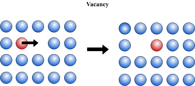
The diffusion of an atom is therefore dependent upon the presence of a vacancy on an adjacent site, and the rate of diffusion is therefore dependent upon two factors: how easily vacancies can form in the lattice, and how easy it is for an atom to move into a vacancy. The dependence upon the presence of vacancies makes substitutional diffusion slower than interstitial diffusion, which we will look at now.
Interstitial Diffusion
In this case, the diffusing atom is not on a lattice site but on an interstice. The diffusing atom is free to move to any adjacent interstice, unless it is already occupied. The rate of diffusion is therefore controlled only by the ease with which a diffusing atom can move into an interstice. Theoretically, at very high impurity concentrations movement may be restricted by the presence of atoms in the adjacent interstices. In practice, however, it is very likely that a new phase would be formed before this had an effect.
Random walk
If we consider an atom undergoing diffusion, we find that we cannot precisely predict its motion. Where the atom is from time to time is essentially random. If there is a preferred direction of motion (perhaps caused by an electric field) then from time to time the atom is more likely to move in that direction. Similarly, if we consider many atoms evenly distributed undergoing diffusion, then their average motion is zero. If there is a preferred direction of motion, we find that there will be a drift in that direction. This random motion can be modelled using a random walk.
One-dimensional random walk
Imagine an atom sitting in an atomic site. The atom will oscillate n times per second, corresponding to a vibration frequency ν. The jump distance, l, is the distance between atomic sites. When left for a time, t, the atom will make a succession of jumps, randomly left or right, and will end up a distance, d, from its starting point. This is known as a “random walk”
For a random walk, the mean distance moved, , is proportional to the root-mean square of the number of jumps made, and therefore to the square root of time:
\[\overline x = \lambda \sqrt n \] \[\overline x = \lambda \sqrt {\nu t} \]
It is significant that we deal with the mean distance travelled. Since the movement of the atom is governed by probabilities, there is a statistical distribution of distances travelled by atoms. For a single atom we cannot know where it will be - only assign probabilities to its potential locations.
This simulation shows the random walk of an atom along a one-dimensional lattice. When there is no bias, there is an equal probability that the atom will move in either direction. If a bias is applied the atom has a greater probability of moving to the right, and statistically is likely to drift in this direction with time.
Two-dimensional random walk
We can now extend this model to a two-dimensional lattice. In this case the atom can move in one of four directions: left, right, up or down, each with an equal probability. As with the one-dimensional lattice, if a bias is applied, the root-mean square distance from the starting point is proportional to the square root of time.
Fick's first law
We have looked at the mechanisms of on an atomic scale. We now want to examine the emergent properties of these mechanisms when there are a lot of atoms. The first thing to note before we start is that no real material has a perfect structure. There will some amount of vacancies or other imperfections present. Therefore if we add impurity atoms to the material, they will be able to move around the material at some rate. If they are interstitial they will move around at a faster rate since they do not require any vacancies to move.
The second thing to note is that if the impurity atoms are distributed evenly throughout the material such that there is no concentration gradient, their random motion will not change the concentration of the material. Nor will there be a net movement of atoms through the material. We are interested in the cases where there is some kind of energy difference in the material, which causes a net movement of atoms. This can be caused by concentration differences, electric fields, chemical potential differences etc.
We will first look at the case of concentration differences. The fact that a concentration difference causes diffusion should be familiar to everyone, particularly in the case of liquids and gases. Consider adding a drop of ink to a bowl of water. The ink will diffuse through the water until the concentration is the same everywhere. There is no force causing the ink particles to diffuse through the water. It is in fact a statistical result of the random motion of the particles.
We can use Fick’s laws to quantitatively examine how the concentrations in a material change.
Consider a crystal lattice with a lattice parameter λ, containing a number of impurity atoms. The concentration of impurity atoms, C (atoms m-3) may not be constant over the whole crystal. In this case there will be a concentration gradient across the crystal, which will act as a driving force for the diffusion of the impurity atoms down the concentration gradient (i.e. from the area of high concentration to the area of low concentration).
Fick’s first law relates this concentration gradient to the flux, J, of atoms within the crystal (that is, the number of atoms passing through unit area in unit time)
Fick’s first law (derivation here) is \(J \equiv - D\left\{ {\frac{{\partial C}}{{\partial x}}} \right\}\)
D is the diffusivity of the diffusing species.
Our equation relating the mean diffusion distance to time can now be modified to be in terms of this parameter:
\[\begin{array}{l} \overline x = \lambda \sqrt {\nu t} \\ D = \frac{1}{6}\nu {\lambda ^2}\\ \overline x = \sqrt {6Dt} \\ \overline x \approx \sqrt {Dt} \end{array}\]
The animation below demonstrates Fick’s 1st Law with respect to a fluid.
Fick's second law
Fick’s second law is concerned with concentration gradient changes with time.
By considering Fick’s 1st law and the flux through two arbitrary points in the material it is possible to derive Fick’s 2nd law.
\[\frac{{\partial C}}{{\partial t}} = D\left\{ {\frac{{{\partial ^2}C}}{{\partial {x^2}}}} \right\}\]
This equation can be solved for certain boundary conditions:
1. “Thin source”
Consider a semi-infinite bar with a small, fixed amount of solute material diffusing in from one end.

The amount of solute in the system must remain constant, therefore\(\int\limits_0^\infty {C\left\{ {x,t} \right\}} {\rm{d}}x = B\), where B is a constant.
The initial concentration of solute in the bar is zero, therefore \(C\left\{ {x,t = 0} \right\} = {C_0}\)
These boundary conditions give the following solution:
\[C\left\{ {x,t} \right\} = \frac{B}{{\sqrt {\pi Dt} }}\exp \left\{ {\frac{{ - {x^2}}}{{4Dt}}} \right\}\]
2. “Infinite source”
A semi-infinite bar with a constant source (i.e. constant concentration) of solute material diffusing in from one end.
In this case, the solution is obtained by stacking a series of “thin sources” at one end of the bar, and summing the effects of all of the sources over the whole bar.
The initial concentration of solute in the bar is C0, therefore \(C\left\{ {x,t = 0} \right\} = {C_0}\)
The concentration of solute at the end of the bar is a constant, Cs, therefore \(C\left\{ {x = 0,t} \right\} = {C_s}\)
These boundary conditions give the following solution:
\[C\left\{ {x,t} \right\} = {C_s} - ({C_s} - {C_0})erf\left\{ {\frac{x}{{2\sqrt {Dt} }}} \right\}\]
erf{x} is known as the error function and results from the summation of the thin sources at the end of the bar. It is defined as
\[erf\left\{ x \right\} = \frac{2}{{\sqrt \pi }}\int\limits_0^x {\exp \left\{ { - {u^2}} \right\}} du\]
The integral can only be solved numerically with a computer, so erf tables are used to solve the diffusion equation where necessary.
This animation shows the applications of Fick’s 2nd law and its solutions.
3. Non-Analytical Solutions
For more complicated situations we cannot obtain an analytical solution for Fick’s 2nd law. In these cases numerical analysis is used. Solutions obtained in this way are approximations, however, they can be made as precise as needed.
The following demonstration shows how numerical analysis can be used to approximate solutions for various conditions.
Interdiffusion
Kirkendall Effect
We will now consider a diffusion couple: that is two semi-infinite bars of materials A and B joined together, such that material diffuses from A to B and from B to A. This is interdiffusion. We can assume that during this process the dimensions of the total bar remain the same, and that no porosity develops.
The diffusivity of the two materials will not be the same: We will assume that DB > DA. This would, in theory, lead to a net drift of atoms towards A; the diffusion couple would appear to move to one side as you look at it!
We know, however, that this does not happen. In practice there is a lattice drift from left to right, so that the bar remains stationary in the laboratory frame. This lattice drift can be detected by placing inert markers at the interface between the two materials, and observing their drift as the two materials interdiffuse. This is known as the Kirkendall effect.
Darken Regime
The Darken equations are Fick's laws adapted for substitutional diffusion, by the motion of vacancies. The equations can be found by equating the flux of atoms and the flux of vacancies within a diffusion couple, and finding the velocity of the lattice drift.
This gives the following equations, known as the darken equation:
\[{J_A}' = - \tilde D\left\{ {\frac{{\partial {C_A}}}{{\partial x}}} \right\}\]
Where \({\tilde D}\) is the interdiffusion coefficient, such that
\[\tilde D = {X_A}{D_B} + {X_B}{D_A}\]
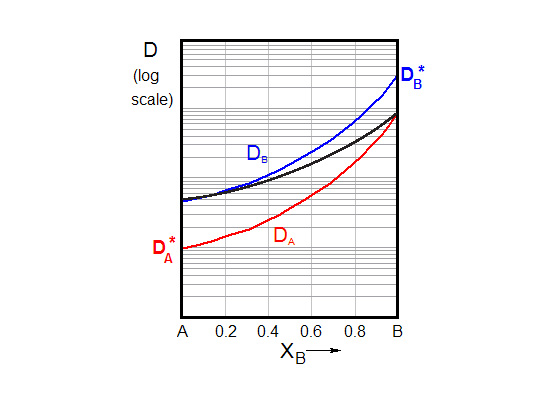
This and the expression for the lattice drift velocity below are known as the Darken relations:
\[v = \frac{1}{{{C_0}}}\left( {{D_A} - {D_B}} \right)\left\{ {\frac{{\partial {C_A}}}{{\partial x}}} \right\}\]
The derivation for this equation is long, and can be found here
Nernst-Planck Regime
The Darken relations only apply if there are sufficient, and efficient, sinks and sources for vacancies, and if diffusion is slow enough, and over large enough distances, that stresses have sufficient time to relax such that no porosity results.
If the sinks and sources are not sufficient, or if the diffusion distance is small (such as in a multilayer), stresses build up, and porosity forms. The Darken regime no longer applies, and the system moves into the Nernst-Planck Regime:
\[\frac{1}{{\tilde D}} = \frac{{{X_B}}}{{{D_A}}} + \frac{{{X_A}}}{{{D_B}}}\]
It is often useful to relate the Darken regime to series conduction, and the Nernst-Planck regime to parallel conduction. In the Darken regime the diffusivity is controlled by the fastest component; in the Nernst-Planck regime it is limited by the slowest.
Microstructural effects
If a material contains grains, the grains will act as diffusion pathways, along which diffusion is faster than in the bulk material.
Consider a cylindrical grain of radius r and grain boundary thickness δ
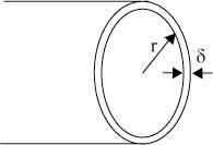
The area of the grain boundary in the cross section is 2π r δ.
Every grain boundary is shared between two grains, so the total grain boundary area associated with one grain is π r δ.
The ratio of the area of the grain boundary to the bulk is:
\[\frac{{\pi r\delta }}{{\pi {r^2}}} = \frac{\delta }{r} = \frac{{2\delta }}{d}\]
The overall flux through unit cross-sectional area is the sum the fluxes through the bulk and the grain boundary:
\[J = {J_\rm{b}} + {J_\rm{gb}}\frac{{2\delta }}{d}\]
The derivation for this equation is here
Therefore:
\[{D_{{\rm{measured}}}} = {D_{\rm{b}}} + {D_{{\rm{gb}}}}\frac{{2\delta }}{d}\]
It is important to realise that δ is very small, therefore grain boundary diffusion only becomes significant when Dgb >> Db, i.e. at low temperatures.
The following animation shows the effect of microstructure on diffusion at various temperatures:
Dislocations have a similar effect, providing fast diffusion paths due to the disruption in the lattice, again with only a significant effect at low temperatures.
Temperature Effects
Enthalpy of migration
In order for atoms to diffuse they must overcome the energy barrier associated with changing their position. The more kinetic energy the atoms have, the more likely it is that the energy barrier will be overcome. The greater the temperature of the system, the greater the kinetic energy of the atoms, therefore temperature has a significant effect on the diffusivity of the species. The energy needed to overcome the barrier is the enthalpy of migration.
For a system with attempt frequency v0 the frequency of successful jumps is given by an Arrhenius dependence:
\[v = {v_0}\exp \left( {\frac{{ - G*}}{{{k_B}T}}} \right)\]
Where ν0 is the pre-exponential, G* is the magnitude of the energy barrier (or the free energy associated with diffusion), KB is Boltzmann’s constant and T is the temperature.
Since
G* = H* - TS*
Where H* = enthalpy of migration and S* = entropy of migration
\[v = {v_0}\exp \left( {\frac{{S*}}{{{k_B}}}} \right)\exp \left( {\frac{{ - H*}}{{{k_B}T}}} \right)\]
Or
\[D = {D_0}\exp \left( {\frac{{ - H*}}{{{k_B}T}}} \right)\]
where \({D_0} = \frac{1}{6}{\lambda ^2}{v_0}\exp \left( {\frac{{S*}}{{{k_{\rm{B}}}}}} \right)\)
which can be assumed to remain constant with varying temperature
H* is often denoted as Q, the activation energy for diffusion.
Enthalpy of vacancy formation
As we have discussed before, the diffusion rate in a substitutional lattice is dependent upon the number of vacancies present, which is also temperature dependent. Therefore, in the case of substitutional diffusion there is a further temperature effect to consider. The equilibrium number of vacancies, Xve, also shows an Arrhenius dependence:
\[{{\rm{X}}_{\rm{v}}}^e = \exp \left( {\frac{{ - \Delta {G_v}}}{{{k_B}T}}} \right)\] \[{{\rm{X}}_{\rm{v}}}^e = \exp \left( {\frac{{\Delta {S_v}}}{{{k_B}}}} \right)\exp \left( {\frac{{ - \Delta {H_v}}}{{{k_B}T}}} \right)\]
Where ΔGv = free energy change on formation of vacancies, ΔSV= entropy change on formation of vacancies and ΔHV= enthalpy change on formation of vacancies.
In the equation to calculate diffusivity, Q can be separated into two components;
- Qm – the enthalpy of migration due to lattice distortions
- Qf – the enthalpy of formation of a vacancy in an adjacent site
Hence
\[D = {D_0}\exp \left( {\frac{{ - {Q_{\rm{m}}}}}{{{k_B}T}}} \right)\exp \left( {\frac{{ - {Q_f}}}{{{k_B}T}}} \right)\]
Since the formation of a vacant site is not needed for interstitial atoms, Qinterstitial << Qsubstitional, and hence Dinterstitial >> Dsubstitional.
Temperature plays a significant role in the rate of diffusion, as it alters the equilibrium concentration of vacancies, and probability of a successful jump into a neighbouring site.
The animation below shows the effect of temperature on both substitutional and interstitial diffusion.
Applications of Diffusion
Diffusion is a key process in much of materials science. We will examine some applications more closely here:
Carburisation
Carburisation is the process by which carbon is diffused into the surface of steel in order to increase its hardness. The carbon forms carbide precipitates (particularly if the steel contains carbide forming elements such as manganese or molybdenum) which pin dislocations and prevent slip, thus making the material harder. However, the increased carbon content reduces the toughness of the material. In most applications it is important that the surface of the steel is hard, but the bulk material can remain softer without detriment to the properties of the component. Thus, carbon is often diffused in from the outer surfaces to obtain a material that is hard on the surface but tough in the bulk.
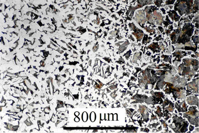
A carburised steel, showing increased carbon content on the outer surface See Micrograph No 289
This is done by heating the steel in a carbon atmosphere, so that there is a concentration gradient of carbon across the interface. Carbon diffuses into the steel, and the elevated temperature speeds up the process. The concentration profile of carbon is governed by Fick’s second law, as there is effectively an infinite source of carbon.
Nuclear Waste
In this case diffusion causes a problem that needs to be solved. Radioactive waste from nuclear energy production must be stored in such a way that the radioactive atoms do not diffuse out of the container until the radioactivity levels have sufficiently dropped. This can be a very long time indeed: often around 1000 years. Thus, the container must be made of a material in which the diffusivity of the atoms is very low (and the container must be very thick, to increase the diffusion distance). This will ensure that the time taken for atoms to diffuse out of the container is as long as possible.
Generally, the radioactive atoms are suspended in a glass matrix, such as borosilicate glass. The diffusivity of the atoms in this glass is low, thus the atoms are less likely to diffuse out of the glass before they have ceased to be radioactive. The glass is then sealed inside steel containers and buried deep in the ground under rocks, in remote areas away from populated regions.
Semiconductors
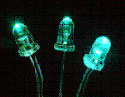
Gallium-Nitride semiconductor LEDs from the Cambridge centre for gallium nitride web site
Semiconductors can be made by doping one material (often silicon) with a small number of atoms of another material of a different valency. This is known as doping, and means that there is an excess of charge carriers in the material (electrons if the valency of the dopant is greater than that of the silicon, or holes if it is less). For more details on this see the TLP on semiconductors.
The doping is often carried out by diffusion methods: the silicon is placed in a gas of the dopant atoms and heated to high temperatures. The dopant atoms diffuse down the chemical potential gradient into the silicon. As with carburisation, this process follows Fick’s second law.
In practice, the diffusion process occurs in two steps. After the initial diffusion described above, the atoms will be concentrated mainly on the surface of the silicon. The sample must therefore be annealed in order to “drive in” the atoms, so that they penetrate beyond the surface.
Summary
In a random walk, the average distance moved from the starting point is proportional to the square-root of time. \(\overline x = \lambda \sqrt {\nu {\kern 1pt} t} \)
Diffusion occurs via two mechanisms, either through the movement of vacancies or interstitial atoms moving between different interstitial sites.
Fick’s 1st and 2nd Laws can be used to calculate the flux of atoms through a crystal structure under different conditions
\[J \equiv - D\left\{ {\frac{{\partial C}}{{\partial x}}} \right\}\;\;{\sf{Fick's}}\;{\sf{1st}}\;{\sf{Law}}\]
\[\frac{{\partial C}}{{\partial t}} = D\left\{ {\frac{{{\partial ^2}C}}{{\partial {x^2}}}} \right\}\;\;{\sf{Fick's}}\;{\sf{2nd}}\;{\sf{Law}}\]
where D is diffusivity
The rate of diffusion varies exponentially with temperature, following the equation;
\[D = {D_0}\exp \left( {\frac{{ - H*}}{{{k_B}T}}} \right)\]
Diffusivity also increases with the vacancy concentration in substitutional diffusion, which means that it is generally higher along grain boundaries and dislocations due to the disruption to the lattice.
Questions
Quick questions
You should be able to answer these questions without too much difficulty after studying this TLP. If not, then you should go through it again!
-
In Fick’s 1st Law, is J (the flux of atoms) proportional to;
-
Which of these diffusion mechanisms is NOT observed?
-
What is Fick’s 2nd Law?
-
What happens to the diffusivity of a material as you increase the temperature?
Going further
Books
- Porter, D.A. and Easterling, K.E., Phase Transformations in Metals and Alloys, Second Edition, Chapman and Hall, 1992.
- Shewmon, P.G., Transformations in Metals, McGraw-Hill, 1969.
- Reed-Hill, R.E. and Abbaschian,,R., Physical Metallurgy Principles, Thrid edition, PWS-Kent Publishing Co., Boston, Mass., 1994.
Websites
- Random walk [http://polymer.bu.edu/java/java/2drw/RandWalk2D.html]
- Random walk [www.compadre.org/osp/items/detail.cfm?ID=8845&Relations=1#tabNav]
- Diffusion [http://www.msm.cam.ac.uk/phase-trans/2001/diffusion.html]
- Kirkendall effect [http://www.msm.cam.ac.uk/phase-trans/kirkendall.html]
Derivation of Fick's first law
Fick’s first law relates this concentration gradient to the flux, J, of atoms within the crystal (that is, the number of atoms passing through unit area in unit time)
Each plane within a crystal will contain Cλ atoms per unit area.
This means that for an increment of distance (δx) of λ, the corresponding increment of concentration (δC) is given by:
\[\partial C = \lambda \left\{ {\frac{{\partial C}}{{\partial x}}} \right\}\]
For a three-dimensional crystal, an atom can move in one of six directions. If the jump frequency is ν, the fluxes of atoms from left to right and from right to left are given by:
\[{J_{L \to R}} = \frac{1}{6}\nu C\lambda \] \[{J_{R \to L}} = \frac{1}{6}\nu (C + \partial C)\lambda \]
Therfore the net flux, J, is given by:
\[ J = {J_{L \to R}} - {J_{R \to L}}\] \[J = - \frac{1}{6}\nu \partial C\lambda \] \[J = - \frac{1}{6}\nu \left\{ {\frac{{\partial C}}{{\partial x}}} \right\}{\lambda ^2}\] \[J \equiv - D\left\{ {\frac{{\partial C}}{{\partial x}}} \right\}\]
This is Fick’s first law: D is the diffusivity of the diffusing species.
Derivation of Fick's second law
Consider a cylinder of unit cross sectional area. We take two cross-sections, separated by δx, and note that the flux through the 1st section will not be the same as the flux through the second section.
From Fick’s first law we can deduce that:
\[{J_1} = - D{\left\{ {\frac{{\partial C}}{{\partial x}}} \right\}_1}\] \[{J_2} = - D{\left\{ {\frac{{\partial C}}{{\partial x}}} \right\}_2}\] \[{J_2} = - D{\left\{ {\frac{{\partial C}}{{\partial x}}} \right\}_1} + \partial x\left\{ {\frac{{{\partial ^2}C}}{{\partial {x^2}}}} \right\}\]
In an increment of time,δt, there is a corresponding increment in concentration, δC.
\[\partial C\partial x = ({J_1} - {J_2})\partial t\] \[\frac{{\partial C}}{{\partial t}} = D\left\{ {\frac{{{\partial ^2}C}}{{\partial {x^2}}}} \right\}\]
This is Fick’s second law
Derivation of darken equation
1. Find the net flux of atoms
From Fick’s first law we can state that:
\[{J_A} = - {D_A}\left\{ {\frac{{\partial {C_A}}}{{\partial x}}} \right\}\] \[{J_B} = - {D_B}\left\{ {\frac{{\partial {C_B}}}{{\partial x}}} \right\}\]
We can assume that the total number of atoms is constant, therefore the two concentration gradients are equal and opposite:
\[\frac{{\partial {C_A}}}{{\partial x}} = - \frac{{\partial {C_B}}}{{\partial x}}\]
Therefore:
\[{J_B} = {D_B}\left\{ {\frac{{\partial {C_A}}}{{\partial x}}} \right\}\]
The net flux of atoms is given by JB − JA, and must be equal to the net flux of vacancies, Jv.
\[{J_v} = \left( {{D_A} - {D_B}} \right)\left\{ {\frac{{\partial {C_A}}}{{\partial x}}} \right\}\]
2. Use this to find the velocity of the lattice drift
The velocity of the lattice drift can be found by relating it to the flux of vacancies, Jv.
In a time increment δt a lattice plane of area A will sweep out a volume Avδt. If there are C0 atoms per unit volume, this volume contains Avδt C0 atoms.
This must be the total number of vacancies passing through the plane, given by Jv Aδt
Thus,
\[{J_v}A\partial t = Av\partial t{C_0}\] \[{J_v} = v{C_0}\]
We now employ the expression for Jv found in section 1:
\[\left( {{D_A} - {D_B}} \right)\left\{ {\frac{{\partial {C_A}}}{{\partial x}}} \right\} = v{C_0}\]
\[v = \frac{1}{{{C_0}}}\left( {{D_A} - {D_B}} \right)\left\{ {\frac{{\partial {C_A}}}{{\partial x}}} \right\}\]
3. Find the effect of this lattice drift on the diffusivity species A and B
From Fick’s first law:
\[{J_A} = - {D_A}\left\{ {\frac{{\partial {C_A}}}{{\partial x}}} \right\}\]
This flux is opposed by the flux due to lattice drift:
Jlatt = ν CA
If JA0 is the net flux:
\[{J_A}' = - {D_A}\left\{ {\frac{{\partial {C_A}}}{{\partial x}}} \right\} + v{C_A}\]
We know v from section 2:
\[{J_A}' = - {D_A}\left\{ {\frac{{\partial {C_A}}}{{\partial x}}} \right\} + \frac{1}{{{C_0}}}\left( {{D_A} - {D_B}} \right)\left\{ {\frac{{\partial {C_A}}}{{\partial x}}} \right\}{C_A}\] \[{J_A}' = - {D_A}\left\{ {\frac{{\partial {C_A}}}{{\partial x}}} \right\} + {X_A}\left( {{D_A} - {D_B}} \right)\left\{ {\frac{{\partial {C_A}}}{{\partial x}}} \right\}\] \[{J_A}' = \left( {{X_A}{D_A} - {X_A}{D_B} - {D_A}} \right)\left\{ {\frac{{\partial {C_A}}}{{\partial x}}} \right\}\] \[{J_A}' = \left( {\left( {1 - {X_B}} \right){D_A} - {X_A}{D_B} - {D_A}} \right)\left\{ {\frac{{\partial {C_A}}}{{\partial x}}} \right\}\] \[{J_A}' = - \left( {{X_A}{D_B} + {X_B}{D_A} + {D_A} - {D_A}} \right)\left\{ {\frac{{\partial {C_A}}}{{\partial x}}} \right\}\] \[{J_A}' = - \left( {{X_A}{D_B} + {X_B}{D_A}} \right)\left\{ {\frac{{\partial {C_A}}}{{\partial x}}} \right\}\] \[{J_A}' = - \tilde D\left\{{\frac{{\partial {C_A}}}{{\partial x}}} \right\}\]
Where \(\tilde D\) is the interdiffusion coefficient, such that
\[\tilde D = {X_A}{D_B} + {X_B}{D_A}\]
Derivation of grain boundary flux equation
Total number of atoms per second = net flux × total area
\[JA = {J_{\rm{b}}}{A_{\rm{b}}} + {J_{{\rm{gb}}}}{A_{{\rm{gb}}}}\]
Dividing all parts by the area of the bulk grain gives;
\[\frac{{JA}}{{{A_{\rm{b}}}}} = \frac{{{J_{\rm{b}}}{A_{\rm{b}}}}}{{{A_{\rm{b}}}}} + \frac{{{J_{{\rm{gb}}}}{A_{{\rm{gb}}}}}}{{{A_{\rm{b}}}}}\]
if Ab >> Agb then A ≈ Ab And so these can cancel in the equation to give;
\[J = {J_{\rm{b}}} + {J_{{\rm{gb}}}}\frac{{2\delta }}{d}\]
Academic consultant: Noel Rutter (University of Cambridge)
Content development: Emily Weal, Jenny Chapman, and Andrew Gibbons
Photography and video: Brian Barber
Web development: Lianne Sallows and David Brook
This DoITPoMS TLP was funded by the UK Centre for Materials Education and the Department of Materials Science and Metallurgy, University of Cambridge.