Nodes, elements, degrees of freedom and boundary conditions

“Nodes”, “Elements”, “Degrees of Freedom” and “Boundary Conditions” are important concepts in Finite Element Analysis.

When a domain (a geometric region) is meshed, it is decomposed into a series of discrete (hence finite) ELEMENTS. The meshed geometry of an exhaust manifold is shown in the figure below. It can be seen that the elements in the mesh conform very well to the geometry, and represent therefore a good approximation of the geometry. The manifold in this instance is meshed with a 3-dimensional brick element which contains 20 NODES. Adjacent elements are connected to each other AT the nodes. A node is simply a point in space, defined by its coordinates, at which DEGREES OF FREEDOM are defined. In finite element analysis a degree of freedom can take many forms, but depends on the type of analysis being performed. For instance, in a structural analysis the degrees of freedom are displacements (U_x, U_y and U_z), while in a thermal analysis the degree of freedom is temperature (T). In the exhaust manifold example, there are 4 degrees of freedom at each node – U_x, U_y, U_z and T, since the analysis is a coupled temperature-displacement analysis (due to thermal expansion effects).  These FIELD VARIABLES are calculated at every node from the governing equation. Field variable values between the nodes and within the elements are calculated using interpolation functions, which are sometimes called shape or base functions.

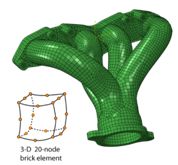
Manifold and node map

There are of course many types of element, covering the complete range of space dimension. The most common are shown in the figure below, along with the position of the nodes, where It can be seen that some of the elements have “midside” nodes – i.e. nodes positioned midway between the corner nodes. The edges of these “higher order” elements can therefore curve – making them suitable for capturing complex geometrical shapes (as in the manifold above). This is possible since these elements permit the solution between the nodes to vary in non-linear ways (see section on shape functions), which is an important feature when field variables change rapidly.

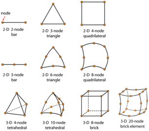
Examples of FEM element types

Boundary Conditions

Boundary conditions are specified values of the field variables (or their derivatives) on the boundaries of the field (the geometry). They fall in to three categories: Dirichlet conditions – where you prescribe the variable for which you are solving; Neumann conditions – where you prescribe a flux, which is the gradient of the dependent variable, and Robin conditions – which is a mixture of the two, where a relation between the variable and its gradient is prescribed. The following table features some examples from various physical fields that show the corresponding physical interpretation.