The Fermi–Dirac Distribution
Electrons are an example of a type of particle called a fermion. Other fermions include protons and neutrons. In addition to their charge and mass, electrons have another fundamental property called spin. A particle with spin behaves as though it has some intrinsic angular momentum. This causes each electron to have a small magnetic dipole. The spin quantum number is the projection along an arbitrary axis (usually referred to in textbooks as the z-axis) of the spin of a particle expressed in units of . Electrons have spin ½, which can be aligned in two possible ways, usually referred to as 'spin up' or 'spin down'.
All fermions have half-integer spin. A particle that has integer spin is called a boson. Photons, which have spin 1, are examples of bosons. A consequence of the half-integer spin of fermions is that this imposes a constraint on the behaviour of a system containing more then one fermion.
This constraint is the Pauli exclusion principle, which states that no two fermions can have the exact same set of quantum numbers. It is for this reason that only two electrons can occupy each electron energy level – one electron can have spin up and the other can have spin down, so that they have different spin quantum numbers, even though the electrons have the same energy.
These constraints on the behaviour of a system of many fermions can be treated statistically. The result is that electrons will be distributed into the available energy levels according to the Fermi Dirac Distribution:
\[f\left( E \right) = \frac{1}{{\exp \left( {\left( {E - \mu } \right)/{k_{\rm{B}}}T} \right) + 1}}\]
where \( f\left( E \right) \) is the occupation probability of a state of energy \( E \), \( k_{\rm{B}} \) is Boltzmann's constant, \( \mu \) (the Greek letter mu) is the chemical potential, and \( T \) is the temperature in Kelvin.
The distribution describes the occupation probability for a quantum state of energy \( E \) at a temperature \( T \). If the energies of the available electron states and the degeneracy of the states (the number of electron energy states that have the same energy) are both known, this distribution can be used to calculate thermodynamic properties of systems of electrons.
At absolute zero the value of the chemical potential, \( \mu \), is defined as the Fermi energy. At room temperature the chemical potential for metals is virtually the same as the Fermi energy – typically the difference is only of the order of 0.01%. Not surprisingly, the chemical potential for metals at room temperature is often taken to be the Fermi energy. For a pure undoped semiconductor at finite temperature, the chemical potential always lies halfway between the valence band and the conduction band. However, as we shall see in a subsequent section of this TLP, the chemical potential in extrinsic (doped) semiconductors has a significant temperature dependence.
In order to understand the behaviour of electrons at finite temperature qualitatively in metals and pure undoped semiconductors, it is clearly sufficient to treat \( \mu \) as a constant to a first approximation. With this approximation, the Fermi-Dirac distribution can be plotted at several different temperatures. In the figure below, \( \mu \) was set at 5 eV.
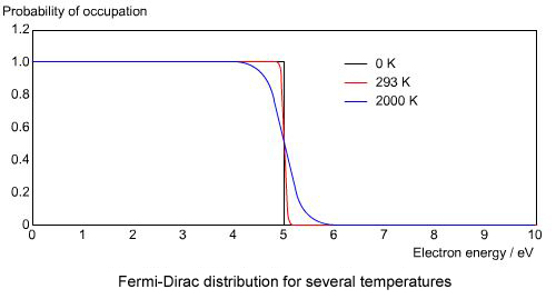
From this figure it is clear that at absolute zero the distribution is a step function. It has the value of 1 for energies below the Fermi energy, and a value of 0 for energies above. For finite temperatures the distribution gets smeared out, as some electrons begin to be thermally excited to energy levels above the chemical potential, \( \mu \). The figure shows that at room temperature the distribution function is still not very far from being a step function.