Superconductivity (all content)

Note: DoITPoMS Teaching and Learning Packages are intended to be used interactively at a computer! This print-friendly version of the TLP is provided for convenience, but does not display all the content of the TLP. For example, any video clips and answers to questions are missing. The formatting (page breaks, etc) of the printed version is unpredictable and highly dependent on your browser.

Contents

Aims

On completion of this TLP you should be able to:

• Know the physical attributes that superconducting materials exhibit;
• Understand the classes of superconductor that exist;
• Have an elementary understanding of the mechanisms that give rise to the properties exhibited by superconducting materials;
• Be familiar with some of the applications of superconductors.

Before you start

This TLP is designed to require minimal previous knowledge. However some knowledge of basic electronic structure and band structure might prove useful. Reading through the TLP on Semiconductors may prove useful before starting this one.

Introduction

The invention of a technique to liquefy helium by Heike Kamerlingh Onnes in 1908 provided scientists with a means of reaching an entirely new range of low temperatures in the vicinity of absolute zero. Helium liquefies at 4.2 K and using this newly accessible range of temperatures to investigate the electrical properties of materials, Onnes found an abrupt drop in electrical resistance where the resistance of the mercury wire he was examining became so low that he could not measure it. This was the first time that anyone had encountered the phenomenon of perfect conduction or “superconductivity”.  In addition, the same class of material was later found to expel magnetic fields.  The combination of perfect conduction and perfect magnetic field expulsion is what defines a superconductor.

The often weird and strange world of quantum mechanics is generally considered to be confined to the atomic level, but with the introduction of superconductivity we actually find a state of matter which exhibits some of the bizarre quantum properties at a macroscopic level. This is what makes superconductivity such an exciting area of study and leads to some new and strange effects.

Discovery and properties

Electrical Resistance – the perfect conductor

Before the successful liquefaction of helium, scientists were unsure about the full temperature dependence of the electrical resistance of metals. It was known that in the region of room temperature, resistance dropped linearly with decreasing temperature. However, as the temperature was lowered this linear relationship failed and the reduction in resistance became smaller. Thus three possibilities were postulated

In fact an entirely different dependence was discovered. Using mercury, which could be easily be made very pure, Onnes discovered that, instead of a smooth transition down to zero resistance that had been proposed, at about 4.2K the resistance of the wire suddenly dropped to below the accuracy of his instruments. The resistance had indeed disappeared and he had discovered a new state, which he named the superconducting state. The temperature at which the transition to superconductivity occurs is known as the critical temperature, T_c.

In order to discover whether the resistance was in fact zero, or just very low, an experiment was designed to measure how long the current would flow in a ring where a current had been induced by a magnetic field. As any measurement of the current would inevitably alter it and introduce some resistance, the magnetic field produced by the flowing current was measured instead.

It has been found that there is no reduction in current over the time period that anyone has had the patience to measure it (the record is over 2  years!). This proved that the resistance was indeed zero.

Many other elements were subsequently found to exhibit a transition from normal to superconducting behaviour at some critical temperature and still more are found to be superconducting if high pressure is applied.

Magnetic Properties – perfect diamagnetism

In 1933 another breakthrough was made in the subject when Meissner and Ochsenfeld started to investigate the magnetic properties of materials as they transitioned from normal to superconducting behaviour. What they found was entirely unexpected and lead to the formulation of a theory that could explain superconductivity.

They observed that when a superconducting material was placed within a magnetic field, the field was completely expelled from the interior of the sample. The ability of a material to partially expel a magnetic field was known already and is called diamagnetism. Almost all materials exhibit some degree of diamagnetism although the effect is usually tiny. In the case of superconductors the effect is large and unexpected.

The phenomenon can be explained by considering a solid sphere of superconducting material. If a magnetic field is then applied, currents are induced in the surface of the sphere, which exactly oppose the applied field and cause no magnetic field to penetrate the sample.

This phenomenon is shown to dramatic effect when a section of superconducting material is placed above a magnetic track. The field from the base is excluded from the superconductor and it levitates. If the superconductor is tapped sideways, it will travel around the track with virtually no resistance to its motion. The video below shows this happening.

Until 1986 it was thought that superconducting behaviour was confined to certain materials at temperatures below ~30 K. A theory called “BCS theory” after its creators John Bardeen, Leon Cooper and Robert Schrieffer had been formulated to describe superconductivity.  This theory, for which its creators received the Nobel Prize in Physics in 1972, appeared to back this up but put a limit on the critical temperature of around 30 K. However, in 1986 a new class of ceramics were discovered to have critical temperatures far in excess of this, much to the amazement of the scientific community. Research into this family of ceramics quickly yielded materials with critical temperatures in excess of 77 K. This breakthrough meant that superconducting behaviour could be observed using liquid nitrogen temperatures instead of the far more expensive liquid helium temperatures that had been used previously. The graph below charts the development of superconducting materials.

Theory

Although superconductivity was discovered as early as 1911, it was not until 1957 that Bardeen, Schrieffer and Cooper postulated a satisfactory explanation of the microscopic mechanism behind the effect.

Two Fluid Model

One of the first models to be formulated to start to describe superconductivity was the two fluid model. This model proposed that electrons within a superconductor appear as two different types, normal and superconducting, i.e. some of the electrons behave as they would in a normal metal and obey Ohm’s law, while others are responsible for the superconducting nature of the material. The crucial aspect of this model is that below Tc, only a fraction of the total number of electrons are capable of carrying a supercurrent. As the temperature is lowered, more of the electrons become the superconducting type while fewer remain as normal electrons.

In the two fluid model, normal and superconducting currents are assumed to flow in parallel when an electric field is applied. However, as the superconducting current flows with no resistance, it will carry the entire current induced by any electric field.

At the time the model was proposed there was no direct evidence for the existence of the superconducting electrons but it did help to explain some of the puzzling experimental observations.

London Conjecture

The next breakthrough in attempting to form an adequate theory came when two brothers, Fritz and Heinz London, made a useful connection between quantum mechanics and superconductivity. They correctly postulated that the diamagnetic properties of superconductors could be described by thinking of the material as a ‘giant atom’ with electrons orbiting around the edges producing the shielding currents responsible for the Meissner effect. This ‘giant atom’ could be produced by having all of the electrons in the body correlated in such a way that the entire specimen could be described by a single wavefunction.

If electrons flow in circulating currents around the surface of a superconductor, they will set up a magnetic field which is equal in magnitude but opposite in direction to the external field applied. This will cause the applied field to be completely expelled and result in the Meissner effect. However, the exclusion of the field from the interior cannot take place exactly up to the surface. This would cause a discontinuous jump in the magnetic field which would require an infinitely large current density at the surface which cannot occur. Thus the magnetic field penetrates the material over a thin surface layer.

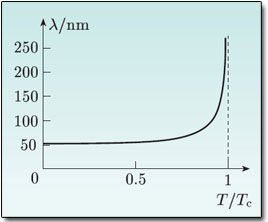
The London equations quantitatively describe these screening currents and the magnetic field in the surface layer. In the simple one dimensional case of a plane perpendicular to the x axis and a magnetic field parallel to the z axis, the magnetic field decays exponentially over a characteristic length, λ.

\[{B_x}(z) = {B_0}{e^{\frac{z}{\lambda }}}\]

Detailed calculations using the London model show that λ is given by \[\lambda = \sqrt {\frac{{{m_{\rm{s}}}}}{{{n_{\rm{s}}}e_{\rm{s}}^2{\mu _0}}}} \]

where m_s, n_s and e_s are the mass, number density and charge of the supercurrent.

This characteristic length, λ, is known as the London penetration depth. A small value of the penetration depth implies that the magnetic field is effectively expelled from the interior of a macroscopic sample. The number density of superconducting electrons is dependent on temperature and means that penetration depth is as well. According to the London model, the penetration depth rises asymptotically as the temperature approaches Tc. Thus the field penetrates further and further as the temperature approaches T_c and does so completely above T_c.

Cooper pairs

In order for electrons to be able to move in some coherent manner and exhibit superconducting properties, there must be some type of interaction between them. Ordinarily, electrons repel each other due to the Coulombic interaction of the similar charge but for electrons to become coherent there must be some type of attraction between them. The breakthrough to describe how there could possibly be an attractive force between two electrons came as a result of experiments looking at the effect of nuclear mass on the critical temperature.

Different isotopes of the same element were found to have different critical temperatures which led scientists to consider the fact that the underlying lattice must have some contribution to the superconducting effect. It was Leon Cooper who came up with the idea that vibrations within the lattice could indeed interact with electrons and cause there to be an attraction between them. The animation below shows the basic mechanism by which this attraction occurs.

Often this pairing of electrons is visualised in terms of ball bearings (the “electrons”) resting on a rubber sheet (the “lattice”). Putting one ball bearing on the sheet will cause it to stretch creating a depression in which the ball sits. This lowers the gravitational potential energy of the ball by making it lower down. If another ball is placed on the sheet, it too will form a depression, but if it is placed near enough to the first the two will roll together and form a deeper depression. This lowers the overall gravitational potential energy of the two balls and causes there to be a coupling between them that would otherwise not be there without the rubber sheet. The animation below gives an idea of how this occurs.  In practice, this is only a schematic representation of the microscopics of the interaction within electron pairs.

Video of the movement of particles into a depression

This analogy can be taken further if we consider the balls to be moving. As the first electron moves it causes the lattice to distort and creates the depression in the rubber sheet. However, the motion of the ball and the relaxation of the rubber sheet occur on different time scales, with the ball moving much faster. This means that there is still a depression in the rubber sheet even after the ball has moved on. This allows the second ball to roll into the well and become effectively bound to the first ball. This is demonstrated by the next animation.

Video of the movement of particles into and out of a depression

Up to now we have considered pairs to be correlated over a fairly short distance. In fact the mean separation at which pair correlation becomes effective is between 100 and 1000 nm. This distance is referred to as the coherence length, ξC_o, of the Cooper pair. This coherence length is large compared with the mean separation between conduction electrons in a metal. Thus Cooper pairs overlap greatly. In between one pair there may be up to 10⁷ other electrons which are themselves bound as pairs.

BCS theory

We are now almost in a position to be able to explain how type I superconductivity arises, but first we need to look at some quantum properties and how electrons are arranged in normal solids and how this differs when the transition is made to the superconducting state.

We know that in normal electronic conduction the electrons that carry the current are scattered by impurities and lattice vibrations that interrupt their motion. In superconductors, however, the superconducting current is carried by Cooper pairs that have to be scattered as a single object without being broken apart. For the electrons which make up the pair to be scattered and produce an interaction we observe as electrical resistance, the Cooper pair must be split apart. This act requires an energy at least equal to the energy gap produced by the binding energy of the Cooper pairs.

Due to random energy fluctuations, even at temperatures below T_c, there will sometimes be enough energy to break the pair and alter the momentum of the electrons. In order to stop the current, however, all of the pairs must be broken which would require a considerable combined effort. As the total energy of the system increases as the temperature is raised and approaches Tc, more and more pairs are broken as electrons are excited above the energy gap. At the transition temperature there are no Cooper pairs left.

Theoreticians often consider the breaking of Cooper pairs as a creation of excitations which consist of electrons which were previously regarded as a bound pair. These “free electrons” are referred to as quasi-particles. At any temperature above 0 K there will be both bound pairs and quasi-particles present. This has striking similarities to the two fluid model which was proposed as a purely phenomenological model.

Type I vs Type II

As scientists began to probe the exciting new properties of superconductors, they discovered that superconductors did have limitations apart from a maximum operating temperature. Although currents can flow without any energy dissipation, superconductivity is destroyed by the application of a sufficiently large magnetic field or if the flowing electrical current density exceeds a critical value.

The critical magnetic field depends on how far below the critical temperature the material is. The graph below shows this dependence.

As more superconducting materials were discovered, it was found that they fell into one of two classes, or “Types” with regard to their magnetic properties, and in particular in the way that they expelled magnetic fields. “Type I” superconductors have a sharp transition from the superconducting state where all magnetic flux is expelled to the normal state.

Type II superconductors, on the other hand exhibit similar behaviour by completely excluding a magnetic field below a lower critical field value and becoming normal again at an upper critical field. However, when the magnetic field is between these lower and upper critical fields, the superconductor enters a “mixed state” where there is partial penetration of flux. In order to lower the overall magnetic energy, the material allows bundles of flux to penetrate the sample. Within these filaments, the magnetic field is high and the superconductor reverts to normal conducting behaviour. Around each of the filaments is a circulating vortex of screening current which opposes the field inside the core. This arrangement ensures that the material outside these bundles remains in the superconducting state. The graph below shows the differing dependence of magnetic field on temperature which characterises type II superconductors.

The so-called flux vortices often arrange themselves into regular periodic structures. They can be visualised by covering the surface with a coagulation of very fine ferromagnetic particles. The animation below shows a micrograph taken of a type II superconductor in the mixed state and how it arises from the partial penetration of flux.

The sample as a whole continues to have zero resistance as current flows by the easiest path and as there are superconducting regions, current can still flow without energy loss. It must be noted however, that if the vortices move they will dissipate energy. For the superconductor to remain lossless, the vortices must be pinned in place by defects within the crystal structure of the material.  Current research aims to understand and pin the resistive motion of flux vortices in applied superconductors, with the aim of creating high critical current materials for applications.

The reason that some superconductors form a mixed state relies on the relationship between the coherence length, ξ, and the London penetration depth, λ. As well as being a description of the distance over which Cooper pairs can be considered to be correlated, the coherence length also describes the distance over which the superconductor can be represented by a wavefunction. For reasons we will not go into, if the penetration depth, λ, is greater than the coherence length, ξ it is thermodynamically favourable for the magnetic field to penetrate the specimen and it will be type II. This is shown schematically in the diagram below.

Relationship between the coherence length and penetration depth for Type I and Type II superconductors

Applications

Power Transmission

One of the most obvious applications of superconductors would appear to be to exploit its zero resistance in making current carrying wires to transport electrical energy. Currently overhead power transmission lines lose about 5% of their energy due to resistive heating. In relative terms this does not seem like a large amount but, due to the vast amount of power that is delivered, this equates to large wastage in real terms.

Clearly this technology has not yet been realised as there are not superconducting wires transmitting power on a commercial scale. A commercially viable superconducting wire must have as high a critical temperature as possible as well as be able to handle significant current densities. However the mechanical properties of the material must also be considered when designing a wire to ensure it is resilient and flexible enough to be used as a replacement for conventional copper wires. This means that the high temperature ceramic superconductors that have recently been discovered are often not yet best suited for this purpose.

In large scale applications, alloys of niobium and titanium tend to be used. These require liquid helium coolant which adds to the cost of running. The wires also have to be much larger than expected in order to avoid what are known as “quenches”. These occur if the wire momentarily stops being superconducting and returns to its normal state. Such a quench creates a region of high electrical resistance and rapidly dissipates a large amount of energy. This can lead to some part of the wire being vaporised, thus destroying the functionality of the wire.

Currently the cost of manufacturing the superconducting wires as well as the cost incurred in maintaining liquid helium temperatures prohibits the use of superconductors in the transmission of power in a commercial environment.

Magnetics

One of the most successful applications of superconductors is in the production of very large magnetic fields. Here superconducting wires are wound into a coil and a high electrical current is passed along the wire in order to produce very high field strengths.

One of the most important applications which require a very high magnetic field is in Magnetic Resonance Imaging (MRI). This technique uses the high field to split the degenerate spin state of a hydrogen nucleus, which can then be investigated using electromagnetic radiation in the radio wave region. This allows the machine to image two dimensional cross sections which have hydrogen atoms in different chemical environments. As the body contains many hydrogen atoms present in water, different tissues in the body give different signals. These two dimensional slices can be built up to form complete pictures of the area of the body being imaged.

Another area which exploits the high field strengths that can be achieved using superconducting magnets is in high energy physics. High strength magnets are key components in particle colliders used to probe the most basic constituents of matter. They are used to deflect high velocity charged particles to keep them in a circle and allow them to be constantly accelerated. High strength magnets are also used in fusion research to contain plasmas. This high temperature state of matter cannot be contained in conventional materials and must be levitated and enclosed using high strength magnets.

Another application making use of superconductors to produce magnetic fields which is already in use is for magnetic levitation (maglev) trains. There are working examples of this technology in use in both Germany and Japan. The animation below outlines the two basic designs of maglev trains and describes how they work.

Electronic Applications

Current microelectronics are beginning to be limited by the speed at which heat can be removed which is produced by the electronic circuits. In order to speed up computing power, interconnects between various components of the circuit can be shortened. However, this creates even more heating problems due to the higher current densities which have to be used. Superconducting wires could eventually be used to remove resistive heating and help solve this problem.

Current silicon based technology is also limited by the speed at which transistors can switch between their 0 and 1 states. Superconducting junctions can be made by exploiting a phenomenon known as the Josephson effect (which is not covered in this TLP) which allows for much greater switching speeds and could greatly increase computer processing speeds.

The Josephson effect is also exploited in making Superconducting Quantum Interference Devices (SQUIDs). These devices allow exceptionally small magnetic fields to be measured and are so sensitive that they can measure the tiny magnetic fields produced by the currents that flow along nerve impulses. This allows for a powerful new technique in neurological research and investigations of the brain.

Summary

This TLP has covered the main aspects of superconductivity:

• The discovery of the superconductive transition at low temperature by Onnes in 1908.
• The properties that define superconductivity – zero resistance and perfect diamagnetism.
• The idea that superconductivity can be explained by a macroscopic quantum state, where electrons move coherently and many can be described by a single wavefunction.
• The London equations which provide a phenomenological model describing the magnetic field penetration within a superconductor.
• The formation of Cooper pairs by the interaction of electrons with lattice vibrations.
• The basics of BCS theory and the creation of an energy gap between filled and unfilled electronic energy levels.
• The difference between type I and type II superconductors with respect to how they interact with external magnetic fields.
• Applications of superconductors and their relevance to everyday life.

Questions

Quick questions

You should be able to answer these questions without too much difficulty after studying this TLP. If not, then you should go through it again!

1. How does the resistance vary with temperature in a perfect superconductor?

   	a	The resistance falls continuously as the temperature approaches absolute zero.
   	b	The resistance initially falls but passes through a minimum before rising as the temperature approaches absolute zero.
   	c	The resistance initially falls before discontinuously dropping to zero at a temperature above absolute zero.
   	d	The resistance falls continuously down to a limiting value as the temperature approaches zero.

2. Which property characterises superconductivity along with zero electrical resistance?

   	a	Perfect Ferromagnetism
   	b	Perfect Paramagnetism
   	c	Perfect Diamagnetism
   	d	The expulsion of any externally applied magnetic field.

3. What carries the current in a superconductor once the electric field is removed?

   	a	Cooper pairs
   	b	Free electrons
   	c	Bound protons

4. What causes electrons in a Cooper pair to be bound together in a conventional superconductor such as Nb or Sn ?

   	a	A coulombic interaction between the electrons
   	b	An interaction between electrons and the vibrations of the lattice
   	c	An interaction between electrons and the external magnetic field

5. How does an externally applied magnetic field interact with a type II superconductor?

   	a	The applied magnetic field is fully expelled by the surface screening currents.
   	b	The applied magnetic field penetrates the material evenly
   	c	The applied magnetic field penetrates the material in 'bundles' which are surrounded by screening supercurrents.

Going further

Books

• Superconductivity – The Next Revolution, Gianfranco Vidali, Cambridge University Press 1993
• Superconductivity, Michael Tinkham, New York: Gordon and Breach 1966
• Superconductivity: Fundamentals and Applications, Werner Buckel, Weinheim: VCH 1991
• Superconductivity of Metals and Cuprates, J.R Waldram, Cambridge University Press 1996

Websites

• University of Birmingham, UK
• National High Magnetic Field Laboratory, USA
• The Open University, UK
• Video Lectures on Superconductivity for SCENET-2 by Dr Bartek Glowacki

Academic consultant: Karl Sandeman (Imperial College, London)
Content development: Henry Begg
Photography and video: Brian Barber
Web development: Lianne Sallows and David Brook

This DoITPoMS TLP was funded by the UK Centre for Materials Education.

Additional support for the development of this TLP came from the Worshipful Company of Armourers and Brasiers'.