Thermal Expansion and the Bi-material Strip (all content)
Note: DoITPoMS Teaching and Learning Packages are intended to be used interactively at a computer! This print-friendly version of the TLP is provided for convenience, but does not display all the content of the TLP. For example, any video clips and answers to questions are missing. The formatting (page breaks, etc) of the printed version is unpredictable and highly dependent on your browser.
Contents
Main pages
Additional pages
Aims
On completion of this TLP you should:
- know how to measure the Young's modulus of a material from the deflection of a cantilever beam made from the material
- understand the origin of the thermal expansion of a solid
- understand how the curvature of a bi-material strip is related to the stiffness of the materials from which it is made and the temperature change it undergoes
- be able to use this relationship to calculate temperature changes and linear expansivities
Before you start
This TLP assumes that you:
- Are familiar with Young's modulus as a measure of the stiffness of a solid material. A definition is provided.
- Are familiar with the concept of the second moment of area (also called moment of inertia).
- Are familiar with the vibrational atomic interpretation of temperature in a solid, and the energy-displacement relationship for atoms in a solid.
Introduction
This TLP is in three parts. The first part involves using the deflection of a cantiliver beam to measure the Young's Modulus of three materials.
In the second part, the origin of thermal expansion in a solid is considered. The relationship between the curvature of a bimaterial strip, the stiffness and thermal expansivities of the materials from which it is made, and the temperature change undergone is examined. The boiling temperature of nitrogen is then estimated by using this relationship and measuring the change in shape of a bimaterial strip made from materials (steel and aluminium) of known thermal expansivities.
In the third part, the previous experiment is repeated with a bi-material strip composed of aluminium and a polybicarbonate. The measured curvature, together with the estimated boiling temperature of nitrogen from the second part, is used to estimate the thermal expansivity of the polycarbonate.
Experiment: Measurement of Young's modulus
View a definition of Young's Modulus.
A cantilever beam is fixed at one end and free to move vertically at the other, as shown in the diagram below.
Geometry of the cantilever beam test.
For each of three strips of material (steel, aluminium and polycarbonate), the strip is clamped at one end so that it extends horizontally, with the plane of the strip parallel to the plane of the bench. A small weight is hung on the free end and the vertical displacement, δ, measured. The value of δ is related to the applied load, P, and the Young’s Modulus, E, by
|
\[\delta = \frac{1}{3}\frac{{P{L^3}}}{{EI}}\] |
(1)
|
where L is the length of the strip, and I the second moment of area (moment of inertia). View derivation of equation.
For a prismatic beam with a rectangular section (depth h and width w), the value of I is given by
|
\[I = \frac{{w {h^3}}}{{12}}\] |
(2)
|
By hanging several different weights on the ends of the strips, and measuring the corresponding deflections, a graph can be can be plotted which allows the Young's modulus to be calculated. This is repeated for each of the three materials. The calculated values for the Young’s modulus may be compared with the values in this properties table.
Experiment to determine Young's modulus
Results: Measurement of Young's modulus
A set of results for the steel strip are given below.
| load, m (kg) |
deflection, δ (10-3 m)
|
| 0 | 0 |
| 0.05 | 3 |
| 0.10 | 6.5 |
| 0.15 | 9 |
| 0.20 | 13 |
| 0.25 | 16 |
A graph of these results gives:
The gradient of this graph is
\[{\rm{gradient}} = \frac{{16 \times {{10}^{ - 3}}}}{{0.25}} = 6.4 \times {10^{ - 2}}{\rm{mk}}{{\rm{g}}^{ - 1}}\]
In addition
| width of strip (w) = | 0.01 m |
| thickness of strip (h) = | 0.001 m |
| length of strip (L) = | 0.15 m |
So, using equation (2)
\[{\rm{gradient}} = \frac{{0.01 \times {{0.001}^3}}}{{12}} = 8.3 \times {10^{ - 13}}{{\rm{m}}^3}\]
From equation (1) with P = mg, a graph of δ against m will have a gradient
\[{\rm{gradient}} = \frac{1}{3}\frac{{g{L^3}}}{{EI}}\]
and hence
\[E = \frac{1}{3}\frac{{g{L^3}}}{{{\rm{gradient}} \times I}} = \frac{{9.8 \times {{0.15}^3}}}{{3 \times 6.4 \times {{10}^{ - 2}} \times 8.3 \times {{10}^{ - 13}}}} = 2.1 \times {10^{11}}{\rm{Pa(2s}}{\rm{.f}}{\rm{.)}}\]
So the steel from which the strip is made has a Young's modulus of 210 GPa (close to the figure given in the properties table).
Repeating the experiment for the aluminium and polycarbonate strips gives Young's moduli of 70 GPa and 5.5 GPa respectively. These results will be used later in the TLP.
Simulation: Measurement of Young's modulus
Origin of thermal expansion
The energy-displacement relationship for atoms in a solid is shown schematically below.
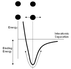
Schematic depiction of the dependence of the potential energy of an atom within a solid on the inter-atomic spacing
As the temperature is raised, the amplitude of vibration increases. The asymmetrical nature of the potential well means that this is accompanied by an increase in the average inter-atomic spacing for longitudinal vibrations. The Coefficient of Thermal Expansion (CTE), or thermal expansivity, α , is the relative change in linear dimensions, per unit of temperature change. In general, ceramics have low thermal expansivities, metals higher and polymers higher still.
Thermal expansivity values for some selected engineering materials, along with some other material data, are given in this properties table.
The bi-material strip
When a component made up of two different materials bonded together is heated or cooled, a misfit is generated between the new dimensions each would adopt if they were isolated. This mismatch can set up stresses and associated distortions. On the other hand, the effect can be exploited by using such a couple to detect or measure temperature changes. An example of such a sensor is the simple bimetallic strip, which has long been used in thermostats and other thermal devices.
As shown in the following diagram, if unbonded the free lengths of each material would be different after a temperature change. When bonded, however, the difference in unconstrained lengths gives rise to internal stresses within the strip, causing it to bend.
The bimaterial strip: (a) Two strips of equal initial length undergo (b) a temperature change ΔT, such that the relative difference in their unconstrained lengths is Δε(= Δα ΔT). (c) Since the two strips are in fact bonded together, the resulting internal stresses generate a uniform curvature. (d) Clamping a bimaterial strip, to allow measurement of the deflection and hence the curvature.
When thermal equilibrium is reached, the resulting curvature, κ, (reciprocal of the radius of curvature) is related to the displacement, >δ, and the distance, x, along the strip at which the displacement is being measured by the relationship
|
\[\kappa = \frac{{2\sin \left[ {{{\tan }^{ - 1}}\left( {{\delta }/{x}} \right)} \right]}}{{\sqrt {\left( {{x^2} + {\delta ^2}} \right)} }}\] |
(3)
|
This can be derived using the geometrical construction shown below.
Geometry for derivation of equation (3)
\[\kappa = \frac{{2\sin \theta }}{{\sqrt {\left( {{x^2} + {\delta ^2}} \right)} }}\]
i.e.
\[\kappa = \frac{{2\sin \left[ {{{\tan }^{ - 1}}\left( {\delta }/{x} \right)} \right]}}{{\sqrt {\left( {{x^2} + {\delta ^2}} \right)} }}\]
The curvature is also related to the material properties and dimensions through the equation
|
\[\kappa = \frac{{6{E_A}{E_B}\left( {{h_A} + {h_B}} \right){h_A}{h_B}\Delta \varepsilon }}{{{E_A}^2{h_A}^4 + 4{E_A}{E_B}{h_A}^3{h_B} + 6{E_A}{E_B}{h_A}^2{h_B}^2 + 4{E_A}{E_B}{h_A}{h_B}^3 + {E_B}^2{h_B}^4}}\] |
(4)
|
where EA, EB are the Young's Moduli, and hA, hB the thicknesses of the two materials A and B. The misfit strain, Δε, is given by
|
Δε = (αA - αB) ΔT |
(5)
|
where αA and αB are the thermal expansivities of the constituents. Derivation of equation (4) is not particularly complex, but need not concern us (see Clyne T W, Key Engineering Materials, vol.116/117 (1996) p.307-330). It is based on the balancing of the bending moment generated by the misfit strain against the opposing moment offered by the beam.
It can be seen that the curvature depends, not just on the expansivity mismatch and temperature change, but also on the relative stiffness and thickness of the two materials. If the two strips are of equal thickness (h), and the stiffness ratio is termed E*, the equation can be re-written
|
\[\kappa = \frac{{12 \Delta \varepsilon }}{{{h_{}}\left( {{E_*} + 14 + 1 / {E_*}} \right)}}\] |
(6)
|
It can be seen that there is a scale effect - i.e. the curvature will be greater when the strips are thinner. Furthermore, a glance at the denominator shows that the curvature will be small if one of the materials has a much greater stiffness than the other.
Assuming the α values for steel and aluminium given in the properties table to be correct, it is possible to use eqns. (3), (5) and (6) to estimate the value of ΔT corresponding to a measured curvature of the steel - Al strip and hence estimate the boiling temperature of liquid nitrogen.
Experiment: Estimating the boiling temperature of nitrogen
A steel tray is used, with a transparent hinged lid, on which a scale is attached.
Steel tray with a transparent hinged lid on which a scale is attached (Click on image to view larger version.)
A steel-aluminium bi-material strip is used, with the two constituent strips having the same thickness and the strips are straight at room temperature. The steel-aluminium strip is fixed securely in the tray, using bolts and wing nuts, locating a spacer block between the side of the tray and the strip, as below.
Arrangement for securing a specimen in the tray
The material with the smaller value of α (steel in this case) is arranged to be closest to the wall of the tray, so that strip will curve away from the nearest wall when cooled.
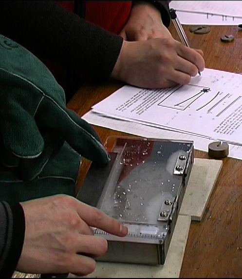
Liquid nitrogen is carefully poured into the tray, so that the strip is partially immersed, avoiding pouring directly onto the strip where possible. It is IMPORTANT that safety glasses and thick gloves are worn throughout this procedure. (Splashing of small amounts of liquid nitrogen onto clothes or skin is not particularly dangerous, but touching very cold metal with unprotected hands can cause severe injury.) The bi-material adopts a uniform curvature, arising from the difference in the free (unconstrained) contractions of each material in the strip. The deflection δ is recorded using the scale on the lid of the tray.
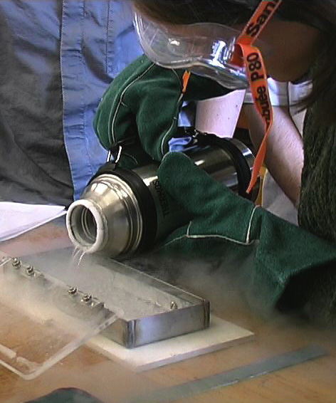
Liquid nitrogen being poured into the tray (Click on image to view larger version.)
Determining the temperature of liquid nitrogen
Results: Estimating the boiling temperature of nitrogen
For the steel-aluminum bi-material strip the following measurements were made
| δ = | 0.021 m |
| x = | 0.189 m |
From equation (3) the curvature
\[\kappa = \frac{{2 \times \sin \left[ {{{\tan }^{ - 1}}\left( {0.021/0.189} \right)} \right]}}{{\sqrt {{{0.021}^2} + {{0.189}^2}} }} = 1.2\]
From equation (6), the misfit strain
\[\Delta \varepsilon = \frac{1}{{12}}\kappa h\left( {{E_*} + 14 + \frac{1}{{{E_*}}}} \right) = \frac{1}{{12}} \times 1.2 \times 0.001 \times \left( {\frac{{210}}{{70}} + 14 + \frac{{70}}{{210}}} \right) = 1.7 \times {10^{ - 3}}\]
And so, from equation (5)
\[\Delta T = \frac{{\Delta \varepsilon }}{{{\alpha _{\rm{A}}} - {\alpha _{\rm{B}}}}} = \frac{{1.7 \times {{10}^{ - 3}}}}{{(1.5 - 2.3) \times {{10}^{ - 5}}}} = - 213{\rm{K}}\]
Given an initial room temperatue of 20ºC, this gives the boiling temperature of nitrogen as 20 - 213 = -193ºC (compare accepted figure of -196ºC).
Experiment: Measuring the thermal expansivity of polycarbonate
First the tray and specimen are brought back to room temperature by immersing in a bucket of water. (Warming up is complete by when the strip has become approximately straight again.)
It is IMPORTANT not to attempt to swap over specimens while the tray is cold.
The experiment is then repeated for the aluminium-polycarbonate strip. The thermal expansivity of polycarbonate can then be estimated, again assuming that the expansivity of aluminium given in the properties table is correct, and using the value for ΔT obtained previously.
Results: Measuring the thermal expansivity of polycarbonate
For the aluminium-polycarbonate bi-material strip the following measurements were made
| δ = | 0.04 m |
| x = | 0.189 m |
From equation (3) the curvature
\[\kappa = \frac{{2 \times \sin \left[ {{{\tan }^{ - 1}}\left( {0.04/0.189} \right)} \right]}}{{\sqrt {{{0.04}^2} + {{0.189}^2}} }} = 2.1\]
From equation (6), the misfit strain
\[\Delta \varepsilon = \frac{1}{{12}}\kappa h\left( {{E_*} + 14 + \frac{1}{{{E_*}}}} \right) = \frac{1}{{12}} \times 1.2 \times 0.001 \times \left( {\frac{{70}}{{5.5}} + 14 + \frac{{5.5}}{{70}}} \right) = 4.7 \times {10^{ - 3}}\]
And so, from equation (5)
\[{\alpha _{\rm{B}}} = {\alpha _{\rm{A}}} - \frac{{\Delta \varepsilon }}{{\Delta T}} = 2.3 \times {10^{ - 5}} - \frac{{4.7 \times {{10}^{ - 3}}}}{{ - 213}}4.5 \times {10^{ - 5}}{{\rm{K}}^{ - 1}}\]
So the thermal expansivity of the polycarbonate material is 4.5 x 10⁻⁵ K-1.
Summary
In this TLP we have:
-
Learned how the Young's modulus of a material may be determined using the relationship between the deflection of a cantilever beam δ and the load P applied to it, given by
\[\delta = \frac{1}{3}\frac{{P{L^3}}}{{EI}}\]
where L is the distance from support to point of load application, I is the second moment of area of the beam's cross section, and E is the Young's modulus of the beam's material.
-
Used measurements of the deflection and load of a steel cantilever beam to determine the Young's modulus of steel as 210 GPa.
-
Looked at how the asymmetry in the energy-separation graph for atoms in a solid gives rise to an increase in the average interatomic spacing of vibrations as the temperature is increased, the origin of thermal expansion.
-
Derived a formula relating curvature κ to the length x and deflection δ of a bi-material strip:
\[\kappa = \frac{{2\sin \left[ {{{\tan }^{ - 1}}\left( {\delta }/{x} \right)} \right]}}{{\sqrt {\left( {{x^2} + {\delta ^2}} \right)} }}\]
-
Defined the misfit strain Δε for the two components of a bi-material strip as
Δε = (αA - αB) ΔT
and quoted a formula relating the curvature κ to the misfit strain, the thickness of the strips h (of equal thickness) and the ratio of the Young's moduli E*
\[\kappa = \frac{{12 \Delta \varepsilon }}{{{h_{}}\left( {{E_*} + 14 + 1 / {E_*}} \right)}}\]
-
Used measurements of the change in shape of a steel-aluminium bi-material strip immersed in liquid nitrogen to estimate the boiling temperature of nitrogen as -193ºC.
-
Used measurements of the change in shape of an aluminium-polycarbonate bi-material strip immersed in liquid nitrogen to estimate the thermal expansivity of the polycarbonate as 4.5 x 10⁻⁵ K-1.
Questions
Quick questions
You should be able to answer these questions without too much difficulty after studying this TLP. If not, then you should go through it again!
-
Which of the following materials has the highest Coefficient of Thermal Expansion (CTE)?
-
In the experiment to determine Young's Modulus, hanging a weight on the cantilever beam leads to a measurement of vertical displacement, d. This value is related to the applied load and the Young's Modulus by the following equation:
\[\delta = \frac{1}{3}\frac{{P{L^3}}}{{EI}}\]
What does I represent in the equation?
-
Which of the following materials has the higher value of Young's Modulus?
-
What do αA and αB represent with respect to materials A and B in the following equation which calculates the misfit strain?
Δε = (αA - αB)ΔT
Deeper questions
The following questions require some thought and reaching the answer may require you to think beyond the contents of this TLP.
-
Explain in terms of atomic structure and bonding why polymers tend to have lower stiffnesses and higher expansivities than metals and ceramics.
-
From the data given in the properties table suggest a suitable pair of metals for the construction of a bimetallic strip. What other factors do you think might in practice be relevant for making such a choice?
Going further
Websites
- Young's Modulus
- From Eric Weisstein's World of Physics, the page considers Young's modulus in the context of elasticity theory.
- Thermal Expansion
- From the thermodynamics part of the HyperPhysics website based at Georgia State University. Includes a section on bimetallic strips, with a video clip of a bimetallic strip being dipped into liquid nitrogen.
- Bimetallic Strip Thermometers
- From the howstuffworks website.
Definition of Young's Modulus
For solids that obey Hooke's Law:
Young's Modulus (E) is the ratio of tensile stress (s) to tensile strain (e) in a specimen subject to uniaxial tension.
\[E = \frac{\sigma }{\varepsilon }\]
This definition then begs for definitions of the terms within it.
For a force tending to elongate a specimen, the tensile stress is the ratio of the *force* (F) applied in a particular direction in the specimen to the cross-sectional area (A) of the specimen in a plane normal to the direction of the applied force.
\[\sigma = \frac{F}{A}\]
(* Strictly speaking, to achieve equilibrium this has to be a pair of equal and opposite forces acting along that direction.)
[If the direction of application of the force is reversed so that the force tends to shorten the sample, the stress is called "compressive".]
If an increment in the tensile stress applied to a specimen of length (l) produces an increment in length (dl) parallel to the direction of application of the stress, the increment in tensile strain (de) is given by
\[\delta \varepsilon = \frac{{\delta l}}{l}\]
and the "true" or "logarithmic" tensile strain (e) is given by
\[\varepsilon = \int_{{l_0}}^{{l_1}} {\frac{{dl}}{l}} = ln\frac{{{l_1}}}{{{l_0}}}\]
For small strains it is often sufficient to approximate the true strain by the "nominal" or "engineering" strain (e)
\[e = \frac{{{l_1} - {l_0}}}{{{l_0}}}\]
Uniaxial tension means that the only externally applied forces acting on the specimen are a pair of equal and opposite forces acting along a line.
Beam deflection during cantilever bending
The beam curvature, κ, is approximately equal to the curvature of the line traced by the neutral axis, d2y/dx2 (see diagram below), so that
\[\frac{{{{\rm{d}}^2}y}}{{{\rm{d}}{x^2}}} = \kappa = \frac{M}{{EI}}\]
where M is the bending moment, E is the Young's modulus and I is the second moment of area. Applying this to the end-loaded cantilever beam, and taking the moment as positive when it generates a displacement in the downward direction (+ive y)
\[EI\frac{{{{\rm{d}}^2}y}}{{{\rm{d}}{x^2}}} = M = F\left( {L - x} \right)\]
where F is the load applied at the end of the beam.
Approximation involved in equating beam curvature to the curvature of the neutral axis (Click on image for larger version)
The deflection is found by integrating this expression, using boundary conditions to establish the integration constants
\[EI\frac{{{\rm{d}}y}}{{{\rm{d}}x}} = FLx - \frac{{F{x^2}}}{2} + {C_1}\] \[{\sf{at }}\;x = 0, \frac{{{\rm{d}}y}}{{{\rm{d}}x}} = 0, \sf{thus}\; {C_1} = 0\]
\[EIy = \frac{{FL{x^2}}}{2} - \frac{{F{x^3}}}{6} + {C_2}\] \[{\sf{at }}\;x = 0, y = 0, \sf{thus}\; {C_2} = 0\]
The deflections along the length of the beam, and specifically at the loaded end, are thus given by
\[y = \frac{{F{x^2}}}{{6EI}}\left( {3L - x} \right)\] \[\delta = \frac{{F{L^3}}}{{3EI}}\]
Mechanical and thermal properties of some engineering materials
| Material |
Young's
modulus (GPa) |
Density
(Mg m-3) |
Thermal
expansivity (K-1 x 10⁻⁶) |
Thermal
conductivity (W m-1 K-1) |
|---|---|---|---|---|
| Mild Steel |
208
|
7.8
|
15
|
60
|
| Aluminium |
70
|
2.8
|
23
|
230
|
| Titanium |
115
|
4.5
|
9.5
|
22
|
| Copper |
117
|
8.9
|
17
|
390
|
| Thermoplastic (e.g. Nylon 6) |
~2
|
1.1
|
~90
|
0.2
|
| Thermoset (e.g. Epoxy resin) |
~3
|
1.3
|
~60
|
0.1
|
| Alumina |
300
|
3.9
|
8
|
30
|
Mechanical and thermal properties of some engineering materials
Academic consultant: Bill Clyne (University of Cambridge)
Content development: Sam Burke, Dave Hudson and David Brook
Photography and video: Brian Barber and Carol Best
Web development: Sam Burke, Dave Hudson and Lianne Sallows
This DoITPoMS TLP was funded by the Higher Education Funding Council for England (HEFCE) and the Department for Employment and Learning (DEL) under the Fund for the Development of Teaching and Learning (FDTL).