X-ray Diffraction Techniques (all content)

Note: DoITPoMS Teaching and Learning Packages are intended to be used interactively at a computer! This print-friendly version of the TLP is provided for convenience, but does not display all the content of the TLP. For example, any video clips and answers to questions are missing. The formatting (page breaks, etc) of the printed version is unpredictable and highly dependent on your browser.

Contents

Aims

On completion of this TLP you should:

• understand the major interactions between X-rays and a crystal lattice
• know how this phenomenon can be used to gain knowledge of the crystalline structure of the material
• be aware of the techniques used to obtain and process X-ray diffraction data

Before you start

You may find it helpful to read the Diffraction and Imaging.

You will find it beneficial to have knowledge of crystal structures, as this will enable a better understanding of the results of X-ray diffraction. This is covered in the Atomic Scale Structure of Materials TLP.

You should also have read the Crystallography TLP and the Lattice Planes and Miller Indices TLP.

Introduction

X-radiation ("X-rays") is electromagnetic radiation with wavelengths between roughly 0.1Å and 100Å, typically similar to the interatomic distances in a crystal. This is convenient as it allows crystal structures to diffract X-rays.

X-ray diffraction is an important tool used to identify phases by comparison with data from known structures, quantify changes in the cell parameters, orientation, crystallite size and other structural parameters. It is also used to determine the (crystallographic) structure (i.e. cell parameters, space group and atomic coordinates) of novel or unknown crystalline materials.

In crystallography, measurements are expressed in Ångströms (Å). An Ångström corresponds to 1 x 10^-10 m; so one Ångström is equal to 0.1 nm.

Experimental matters

Production and measurement of X-Rays

The laboratory source of X-rays consists of an evacuated tube in which electrons are emitted from a heated tungsten filament, and accelerated by an electric potential (typically several tens of kilovolts) to impinge on a water-cooled metal target. When the target’s inner electrons are ejected and outer ones fall to take their place, X-rays are emitted. Some have a continuous distribution of wavelengths between about 0.5 Å and 5 Å ("white radiation") and some have wavelengths characteristic of the electronic levels in the target. For most experiments, a single characteristic radiation is selected using a filter or monochromator.

Methods for obtaining Characteristic Radiation

The diagram below illustrates the characteristic X-ray emission spectrum that is obtained from a copper target.

The white and K_β radiation can be reduced by

1. Using a filter which works by the absorption principle:

The Ni absorption edge is midway between the K_ß and K_a lines so that the former is reduced very substantially while the latter is only marginally reduced.. In selecting the thickness of the filter, a compromise has to be reached between eliminating as much as possible of the undesired radiation and maximising the desired radiation.

For other wavelengths other elements will provide suitable filters.

2. A monochromator that works on the principle of diffraction: 

During diffraction a monochromator (a single crystal of known lattice spacing and orientation) is placed in the path of the primary or diffracted beam. The monochromator is set so that the beam is diffracted and only X-rays with the required wavelength reach the detector. (See Bragg’s law).

3. Modern detectors also filter wavelengths (or energy) electronically

Detectors

In the past most X-ray work was done with film, now electronic detectors are used. A single point (e.g. Geiger Muller, scintillation or proportional counter), a line (1D) or an area (2D) detector may be used.

Bragg′s law

The concept used to derive Bragg's law is very similar to that used for Young’s double slit experiment.

An X-ray incident upon a sample will either be transmitted, in which case it will continue along its original direction, or it will be scattered by the electrons of the atoms in the material. All the atoms in the path of the X-ray beam scatter X-rays. We are primarily interested in the peaks formed when scattered X-rays constructively interfere. (In addition, after scattering some X-rays suffer a change in wavelength. This incoherent scattering is not considered here).

Constructive interference occurs when two X-ray waves with phases separated by an integer number of wavelengths add to make a new wave with a larger amplitude.

When two parallel X-rays from a coherent source scatter from two adjacent planes their path difference must be an integer number of wavelengths for constructive interference to occur.

Path difference = n λ

Therefore;

n λ = 2 d sin θ

In order to consider the general case of hkl planes, the equation can be rewritten as:

λ = 2 d_hkl sin θ_hkl

since the d_hkl incorporates higher orders of diffraction i.e. n greater than 1.

The angle between the transmitted and Bragg diffracted beams is always equal to 2θ as a consequence of the geometry of the Bragg condition. This angle is readily obtainable in experimental situations and hence the results of X-ray diffraction are frequently given in terms of 2θ. However, it is very important to remember that the angle used in the Bragg equation must always be that corresponding to the angle between the incident radiation and the diffracting plane, i.e. θ.

The diffracting plane might not be parallel to the surface of the sample in which case the sample must be tilted to fulfil this condition. (The concept of orientation will be dealt with later in this TLP).

This is the procedure to obtain asymmetric reflections and work in transmission:

Single crystal diffraction

The simplest way of demonstrating application of Bragg’s law is to diffract X-rays through a single crystal.

The simple teaching diffractometer in the photo below projects a beam of X-rays onto the crystal. The diffracted beam is collated through a narrow slit and passed through a nickel filter. The counter is a Geiger-Müller tube.

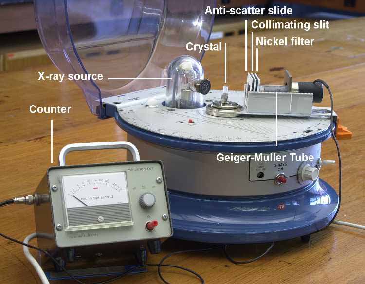
Diffractometer (Click on image to view larger version)

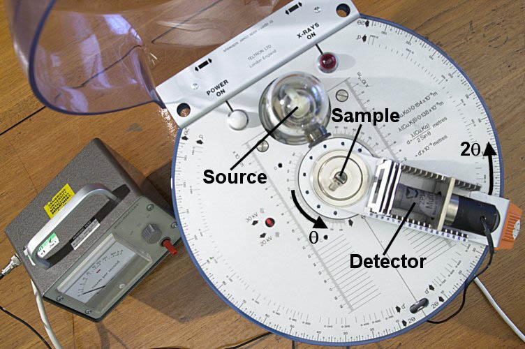
Top view of diffractometer (Click on image to view larger version)

The crystal used in this experiment is lithium fluoride. Assuming that the large flat face will be perpendicular to a particular crystallographic direction, this is set parallel to the line containing the source and detector at θ = 0.  The gearing of the counter arm is such that, once set, the θ - 2θ relationship between the incident, transmitted and diffracted beams is maintained.

The video below shows manual operation and the location of the first diffraction peak. Watch the counter carefully.

Diffractometer experiment with lithium fluoride crystal

Using the 2θ value observed at a peak of intensity, the known wavelength λ for Cu Ka, = 1.54Å and the Bragg equation, a value for the plane spacing (d spacing) can be determined. If the peaks can be indexed, i.e. assigned to scattering from certain planes, then from simple geometry lattice parameters can be calculated. This is shown later in the TLP.

Determining lattice parameters accurately

When using diffraction data to obtain a lattice parameter, it is important to note the shape of the θ - sin θ curve:

The largest gradient on this curve is at low values of θ. This means that a small error in the recorded angle of the diffraction peak will cause a significant error in the calculated lattice parameter. At high values of θ the error in the calculated sin θ value will be reduced. This leads to a smaller error in the calculated value of the lattice parameter. The same conclusion can be drawn by differentiating the Bragg equation.

This implies that lattice parameters calculated from high angle diffraction peaks are more accurate than those taken from low angle peaks.

Relationship between crystalline structure and X-ray data

Peak positions

Using Bragg's Law, the peak positions can be theoretically calculated.

\[\theta = \arcsin \left( {\frac{\lambda }{{2d}}} \right)\]

For a cubic unit cell:

d = \(\frac{a}{{\sqrt N }}\), where N = h² + k² + l² and a is the cell parameter.

(More complex relationships for less symmetrical cells are given in most standard text books)

So the measured value 2θ can be related to the cell parameters.

In the earlier video peak was observed at about 44.4. Knowing the wavelength, 1.54Å, and using Bragg's Law gives a d-spacing of ~2.04 Å. Some additional information is required to obtain lattice parameters from this d-spacing. Knowing that LiF has a cubic structure with a unit cell ~4.03, means that this reflection must be (002) (which is the same as (200) and (020)).

Peak intensities

The structure factor, F_hkl, of a reflection, hkl, is dependent on the type of atoms and their positions (x, y, z) in the unit cell.

\[{F_{hkl}} = {\sum\limits_i {{f_i}} _{}}\exp 2\pi i(h{x_i} + k{y_i} + l{z_i})\]

f_i is the scattering factor for atom i and is related to its atomic number.

The intensity of a peak I _hkl is given by:

\[{I_{hkl}} \propto {\left. {\left| {{F_{hkl}}} \right.} \right|^2}\]

The proportionality includes the multiplicity for that family of reflections and other geometrical factors.

Differences in intensity do relate to changes in chemistry (scattering factor). However, most commonly for multiphase samples, changes in intensities are related to the amount of each phase present in the sample. Suitable calibration factors are required to perform quantitative phase analysis.

Peak widths

The peak width β in radians (often measured as full width at half maximum, FWHM) is inversely proportional to the crystallite size L_hkl perpendicular to h k l plane.

\[{L_{hkl}} = \frac{\lambda }{{\beta \cos \theta }}\;\;\;\;\;\; \rm{Scherrer\;\; equation} \]

(Whilst small crystals are the most common cause of line broadening but other defects can also cause peak widths to increase.)

In the next section there is a simulation which shows how changes in the structure of a simple cubic material influences the diffraction pattern.

Powder diffraction

A powder is a polycrystalline material in which there are all possible orientations of the crystals so that similar planes in different crystals will scatter in different directions.

Scattering in X-ray powder diffraction

In single crystal X-ray diffraction there is only one orientation. This means that for a given wavelength and sample setting relatively few reflections can be measured: possibly zero, one, two (as in the video) or possibly up to say three or four. As other crystals are added with slightly different orientations, several diffraction spots appear at the same 2θ value and spots start to appear at other values of 2θ. Rings consisting of spots (spotty rings) and then rings of even intensity are formed. A powder pattern consists of rings in 2-dimensions, and spheres in 3-dimensions, of even intensity from each accessible reflection at the 2θ angle defined by Bragg's Law.

The other situation which is intermediate between single crystal and powder diffraction is when the sample is oriented and the spots are spread into arcs. This is covered later in the TLP.

This animation shows the relationship between single crystal and powder diffraction, as measured on a 2-dimensional detector (such as film):

An X-ray diffractometer

The photograph below shows a typical powder diffractometer

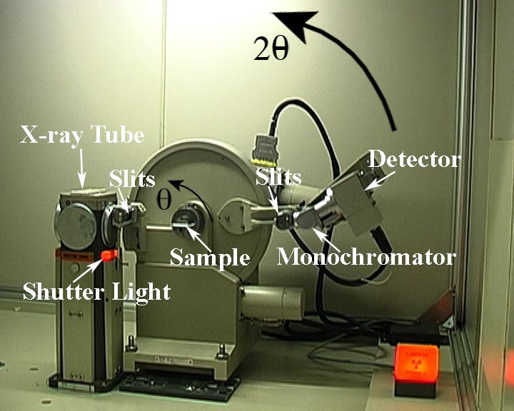
The X-ray beam comes from the tube, through slits, is diffracted from the sample, goes through another set of slits, diffracted from the secondary beam monochromator and measured by the detector.

The video below shows how the sample moves through θ (~5 to 45 ° ) while the detector scans through 2θ (~10 to 90 ° ). It has been speeded up as typical data collection time would be somewhere between 10 mins and 10 hours.

The simulation below shows how the powder diffraction pattern of a simple face-centred cubic structure is influenced by changes in the cell parameter, atomic number, crystallite size and what happens when the material becomes amorphous.

Phase identification

Phase Identification

Powder diffraction data are commonly used to identify or ‘finger print’ crystalline materials. An international database was started in the 1930s and is regularly updated.

In its simplest form, PDF1 (powder diffraction file) lists d-spacings and relative intensities. Most data are now indexed and so include cell parameters, the chemistry, density and other properties of the material. This is called PDF2. It is maintained by ICDD (International Centre for Diffraction Data) formerly JCPDS (Joint Committee for Powder Diffraction Standards).

To identify a particular phase both peak positions and relative intensities must fit. In general this requirement should hold for at least three peaks. Below are two examples of how this process works. The first one is a simple purity check on hydroxyapatite and the second a more complex example identifying three possible phases in stabilised zirconias. Similar logic applies to completely unknown samples.

Oriented (or textured) samples

These can be considered as intermediate between single crystal and powder samples. In a diffractometer scan the relative intensities of the peaks are intermediate between those of a single crystal and a powder. The change in relative intensities may indicate the orientation of the sample. This can be observed in the following simulation:

In a complementary manner, orientation can be measured by recording how a reflection is spread at constant 2θ. An unoriented powder has rings of constant intensity, while an oriented sample has an arc or sharp spot.

It is sometimes helpful to consider oriented samples in reciprocal space.

Summary

Following completion of this TLP, you should have a basic understanding of the phenomenon of X-ray diffraction through a crystalline material. This package has explained how to use an X-ray diffraction experiment to reveal information such as what crystalline phases are present, their cell (or lattice) parameters, crystallite size and whether the phase is single crystal, oriented or a polycrystalline powder. The main aspects of collecting and analysing X-ray data in the laboratory have been covered.

Questions

Quick questions

You should be able to answer these questions without too much difficulty after studying this TLP. If not, then you should go through it again!

1. In a simple X-ray scan, which of these affects the peak positions?

   Yes	No	a	X-ray wavelength
   Yes	No	b	Crystallite Size
   Yes	No	c	Unit cell parameter
   Yes	No	d	Atomic number

2. Which of these is not involved in the diffraction of X-rays through a crystal?

   	a	Electron Scattering
   	b	Crystallographic planes
   	c	Nuclear interactions
   	d	Constructive interference

3. What is the smallest d-spacing that can be measured for a given wavelength λ?

   	a	0.5λ
   	b	λ
   	c	2λ
   	d	no limit

Deeper questions

The following questions require some thought and reaching the answer may require you to think beyond the contents of this TLP.

4. What sort of improvement in precision might you expect in cell parameter calculations when increasing 2θ?

5. A crystal has a cubic unit cell of 4.2 Å. Using a wavelength of 1.54 Å at what angle (2 θ) would you expect to measure the (111) peak ?
   a. 10.6º
   b. 18.5º
   c. 43.0º
   d. 37º

6. For a sample with a crystallite size of 100Å and using a wavelength of 1.54 Å estimate the peak breadth, in radians and degrees, of a peak at 60° 2θ.

7. Given these experimental and reference data (A,B,C and D) which phases are:
   1. Definitely present
   2. Not observable (implies absent at any significant level)
   3. Unsure
   In each case give a reason for your answer and when unsure consider whether you could do something to clarify the situation.
   

Going further

Books

• C. Hammond, The Basics of Crystallography and Diffraction, 2nd edition, OUP, 2001
• B. D. Cullity and S. R. Stock, Elements of X-ray Diffraction, 3rd edition, Prentice Hall, 2001

Websites

• Reciprocal Lattice TLP on using reciprocal space to understand diffraction patterns.
• A detailed interactive tutorial about diffraction. Created by the Universities of Würzburg and Munich.
• International Union of Crystallography (IUCr) The ultimate reference for crystallography. Also has links to many other crystallographic websites.
• CCP14. This site primarily hosts crystallographic software but also has links to web based teaching resources
• Advanced Certificate in Powder Diffraction on the Web.
• Interactive course on crystallography. Created at EPFL, Switzerland. This course introduces the basic concepts of crystallography and is freely available on the web for everyone. The symmetry of crystalline material and the properties of diffraction are presented by means of interactive applets. The description of structures is greatly facilitated by the combination of drawing tools and easy access to databases.

Academic consultant: Mary Vickers (University of Cambridge)
Content development: T D Skinner
Photography and video: Brian Barber and Carol Best
Web development: David Brook

This DoITPoMS TLP was funded by the UK Centre for Materials Education and the Department of Materials Science and Metallurgy, University of Cambridge.

Additional support for the development of this TLP came from the Worshipful Company of Armourers and Brasiers'.