Powder processing (all content)

Note: DoITPoMS Teaching and Learning Packages are intended to be used interactively at a computer! This print-friendly version of the TLP is provided for convenience, but does not display all the content of the TLP. For example, any video clips and answers to questions are missing. The formatting (page breaks, etc) of the printed version is unpredictable and highly dependent on your browser.

Main pages

Aims
Before you start
Introduction
Powder particles in a fluid stream
Particle size measurement by light scattering
Particle impact on substrates
Case study - thermal spraying
Passage of particles through filter
Diesel particulate filters
Powder consolidation by cold pressing and sintering
Summary
Questions
Going further

Additional pages

Reynolds number
Stokes law
Fraunhofer scattering
Stokes number
The Carman-Kozeny Equation
DPF Materials

Aims

On completion of this TLP you should:

Understand the factors that control the dynamics of solid particles in fluids
Be familiar with the main method for measurement of particle size distribution
Be able to make simple calculations relating to the flow of fluids through permeable media, such as filters
Understand how powders are commonly handled and processed to make solid artefacts or surface coatings

Before you start

There are no special prerequisites for this TLP.

Introduction

Handling and processing of powders is central to many areas of science and technology. Most ceramic materials can only be formed via powder processing, but powder metallurgy is also an important branch of materials science and polymers are frequently handled as (coarse) particles. Powder processing is also pivotal in many other industrial sectors, such as food, pharmaceuticals, agriculture, mining etc. Moreover, an understanding of the behaviour of assemblies of solid particles in fluids is essential in areas as diverse as filtration of Diesel exhaust and avoiding explosions in flour mills. Particle sizes of interest vary from a few nm to several mm (although most technological activity is focussed on the range from 100 nm to 100 microns).

Important background includes the factors affecting the dynamics of solid particles suspended in fluids and the flow of fluids through porous mdia (including filters). This TLP provides an introduction to the equations and dimensionless numbers that control these effects, with simulations that allow the behaviour to be explored in particular cases. There are also sections dealing with measurement of particle size and the procedures involved in consolidation of powder particles into solid articles, via various types of sintering process, and the creation of surface coatings via thermal spraying of particles.

Powder particles in a fluid stream

Particles in a fluid can experience several different types of force. The main ones are: (a) Gravitational / Buoyancy (usually due to the particle being more dense than the fluid, creating a force in the direction of a gravitational, or centrifugal, acceleration), (b) Drag (Viscous) (a velocity difference between particle and fluid leading to a drag force acting to reduce this difference) and (c) Electrostatic (due to particles becoming electrically charged and experiencing forces if electric or magnetic fields are present).

A key characteristic of fluid flows is the Reynolds number, Re, representing the ratio of inertial to viscous forces. Low values (Re < ~10 – 500) imply that viscous forces predominate, so that flow tends to be laminar and smooth, whereas large values lead to turbulence, with chaotic eddies and instabilities. An expression for the Reynolds number, and some comments about its magnitude, are provided here.

For laminar flow, the basic equation of fluid motion (the Navier-Stokes equation) can be solved to give Stokes law (relating the frictional (drag) force on a body to its size and relative velocity in a fluid), which is provided here.

By setting this force equal to the net gravitational force, the steady state (terminal) velocity of a (spherical) body falling under gravity in a static fluid can be obtained as:

\[{u_{{\rm{ter}}}} = \frac{{{d^2}\Delta \rho g}}{{18\eta }}\]

where Δρ is the difference in density, d is the particle size, g is the acceleration due to gravity and ν is the viscosity of the fluid. For a typical (ρ ~ 4000 kg m^-3) powder particle, of diameter 100 μm, falling freely in air, this velocity is about 1 m s^-1. Of course, for smaller particles it is much lower (u_ter ~ 0.1 mm s^-1 for 1 μm diameter), so that such fine particulate has a very slow sedimentation rate and readily tends to become, and remain, airborne. The simulation below allows exploration of terminal velocity values for various cases, and also shows how this velocity is approached by a particle that is initially at rest in the fluid. Once 'Start' has been clicked, the particle size and density, and the type of fluid, can be changed while the simulation is running, which may be helpful in exploring the sensitivity of the behaviour to these variables.

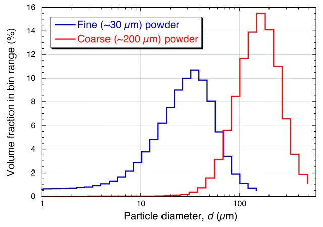
Provided below are four short videos, showing the outcome of inverting small transparent containers in which there are particles suspended in a liquid. For two of them, the liquid is water, while for the other two it is (rapeseed) oil. In each case, there are either small (average diameter ~ 30 µm) or large (average diameter ~ 200 μm) particles present in the liquid. (The size distribution for these two sets of particles is shown at the end of this page: the particles are volcanic ash, with a density of about 2.5 Mg m^-3, so that Δρ is in all cases ~ 1.5 Mg m^-3)

For coarse particles in water, the terminal velocity is ~ tens of mm/s, so particles pass though the field of view in about a second or so and it takes less than a minute for essentially all of the particles to have fallen to the base of the container.

Coarse particles in Water (Viscosity ~ 10^-3 Pa s) - u_ter ~ 30 mm s^-1

With finer particles, the terminal velocity is ~ 1 mm/s. Particles now take something like 20 s to pass though the field of view and they are more susceptible in the initial period to being carried upwards by the convection currents. In this case, it takes several minutes for the liquid to become clear.

Fine particles in Water (Viscosity ~ 10^-3 Pa s) - u_ter ~ 1 mm s^-1

The rapeseed oil has a much higher viscosity than water, so even the coarse particles sediment slowly, taking several tens of seconds to pass through the field of view and it takes about 20 minutes for the liquid to become clear again.

Coarse particles in Oil (Viscosity ~ 5 10^-2 Pa s) - u_ter ~ 0.5 mm s^-1

Fine particles in the oil have a very low terminal velocity (of a few tens of microns per second). They can take periods of a minute or more to pass through the field of view, and in fact it can be seen that particles can readily be carried upwards by convection currents. However, another effect is also apparent here - there is a tendency for these fine particles to clump together in this viscous liquid and relatively dense agglomerates of this type behave differently, tending to fall with a higher velocity, in a similar way to that expected with much larger particles.

Fine particles in Oil (Viscosity ~ 5 10^-2 Pa s) - u_ter ~ 0.02 mm s^-1

The Particle Size Distributions for the two powder samples in the above videos are shown below. (These were obtained by Laser Scattering - see the next page.)

Particle size measurement by light scattering

There are several techniques for measuring the Particle Size Distribution (PSD) of a powder, but the most popular is based on the way that particles scatter light, which depends on their size. Such scattering is very commonplace. A light beam passing through a column of smoke is reduced in intensity, but little of this reduction is due to actual absorption of light by the particles and, if the column were to be viewed from the side in a darkened room, it would be clear that most of the "lost" light is being scattered sideways. This is mainly Fraunhofer scattering, similar to that emerging from a narrow slit. The corresponding equation is provided here.

Measurement of the intensity of light scattered from a dispersion of particles, as a function of scattering angle, thus allows the particle size distribution (PSD) to be deduced. Particles are normally dispersed in a liquid, which may need to be continuously stirred, and laser light is used, giving high incident intensities at a fixed wavelength. Software is supplied that allows the PSD to be automatically produced after a short time (~1 minute) of measurement.

The range of particle size for which this technique is reliable is from around 1 μm up to ~100 μm, which is satisfactory for many powders. The presence of smaller particles can be analysed via the effect that Brownian motion has on them, creating small fluctuations in the intensity of light scattered through large angles. These fluctuations can be detected, allowing measurement of particles down to about 0.1 μm, although specialised experimental set-ups are required for this.

The image below shows a set-up for measurement of PSD via scattering of laser light (http://www.lsinstruments.ch/technology/small_angle_light_scattering/)

Set-up of PSD via scattering of laser light

The two videos below were obtained using a set-up similar to that shown above, with the two powders used in the previous page suspended in rapeseed oil. (As indicated there, these particles remain in suspension for extended periods.) The first shows the outcome with the coarser particles. It can be seen that most of the scattered light is being diffracted through an angle of about 0.2-1˚, which is broadly consistent with the Fraunhofer equation (see above). The stochastic nature of the scattering events is apparent in this video.

Laser Scattering with 200 μm particles in suspension

The corresponding video for the 30 μm powder particles can be seen below. It can be seen that the average scattering angle is now somewhat larger - up to about 2˚, again in approximate agreement with the Fraunhofer equation. Also, while there are again random fluctuations as the individual particles tumble through the laser beam, the fact that they are finer, and there are more of them, leads to a slightly more uniform and constant image than with the coarser particles.

Laser Scattering with 30 μm particles in suspension

Particle impact on substrates

The likelihood of a particle in a fluid stream striking a solid obstacle depends on the Stokes Number, Stk, which is the ratio of the characteristic time needed for the particle to change its velocity to that needed for it to pass the obstacle. If Stk>>1, then particles will strike the obstacles, while Stk<<1 means that most particles are expected to pass around them within the fluid stream. Derivation of the expression for the Stokes number is provided here.

It can be seen from the expression for Stk that particle size is important, with finer particles more likely to be carried around an obstacle without striking it, while coarser (and more dense) particles cannot change their velocity so quickly and are likely to carry on in a straight line, so that impact occurs. Fluid velocity and viscosity are also relevant, with high velocity and low viscosity also favouring impact. These effects can be quantitatively explored in the simulation shown below - click on "start" to inject the particles, after setting the parameter values. (Note that the substrate (obstacle) size in this simulation is fixed at the rather low value of 0.3 mm, and the velocity range is only up to 1 m/s: in the next page, this formulation is used in a simulation of thermal spraying, in which a high velocity air stream carries particles towards a substrate.)

Case study - thermal spraying

Thermal spraying is widely used to produce high quality coatings, mostly ceramic or metallic, and, to a lesser extent, for purposes of repair or to build up a shaped component. It is most commonly carried out by feeding powder into a high temperature, high velocity gas stream, where the particles gain heat and momentum (and may or may not closely approach the temperature and/or velocity of the surrounding gas).

Particles are carried by the gas stream towards a substrate, on which they are expected to impinge, deform and adhere. The issue of whether a particle in a fluid stream is likely to strike an obstacle is covered in the previous page: it's controlled by the Stokes number. As explained there, very fine particles are unlikely to strike surfaces. During thermal spraying, velocities are quite high (u ~100 m s^-1), favouring impact, but obstacles (substrates) are relatively large (D >~10 mm), with the opposite effect (giving the particle more time to change direction). An estimate of minimum particle size for impact (by setting Stk ~ 1), for a particle with a typical density (~3 × 10³ kg m³), is given by

\[{d_{\min }} \approx \sqrt {\frac{{18\pi D}}{{\Delta \rho u}}} \approx \sqrt {\frac{{18({{310}^{ - 5}})(0.01)}}{{(3 \times {{10}^3})(100)}}} \approx 5\mu {\rm{m}}\]

In general, therefore, thermal spraying is not carried out with fine particles and a typical size range would be ~20-100μm.

The treatment on the previous page can also be used to explore times and distances over which particles will be accelerated to velocities close to that of the gas (which may itself be dropping off with distance ahead of the torch). The expression (for the characteristic time for a particle to change its velocity (so that it's close to that of the gas) leads to times of ~10 ms and 40 ms for particle diameters of 50 μm and 100 μm. Gas velocities in thermal spraying range from several tens of m s^-1 to (supersonic) speeds of several hundred m s^-1. Taking 100 m s^-1 as representative, the distances needed for particles with these two sizes to approach that speed (assuming linear acceleration over the above periods) are about 0.5 m and 2 m. This is, of course, a crude estimate, and there is no need for the particle velocity to closely approach that of the gas, but it does show that a relatively large "stand-off" distance may be needed for particles to reach peak velocity.

The other main issue is heat transfer from gas to particle. This is complex, but can be simplified by use of a heat transfer coefficient (interfacial thermal conductance), h_i, which relates the heat flux into a particle to the temperature difference between particle surface and nearby gas. The value of h_i can be expressed as K_g / δ, where K_gis gas conductivity and δ the thickness of a thermal boundary layer in the gas around the particle. The value of δ depends on relative velocity, gas viscosity, particle size and shape etc, so generalisations are difficult. Typically, however, h_i ranges from ~100 kW m^-2 K^-1 (fine particle, high relative velocity) to ~1 kW m^-2 K^-1 (coarse particle, low relative velocity). Since K_g for most gases is ~0.02 W m^-2 K^-1, corresponding boundary layer thicknesses are ~0.2 μm and ~20 μm.

A value of hi allows estimation of heating rates, and also of whether particles remain isothermal or develop large internal thermal gradients. The latter can be decided from the value of the Biot number (ratio of conductance of interface to that of the particle):

\[{\rm{Bi }} \approx \frac{{{h_i}}}{{K/L}} \approx \frac{{{h_i}(d/2)}}{{{K_p}}}\]

Using the figures above, and taking K_p to be ~5 W m^-2 K^-1 (ceramic), Bi for a fine particle (d~5 μm) is ~0.05, while for a large particle (d~100 μm) it is ~0.01. These are both <<1, implying that all (thermally-sprayed) particles remain isothermal during the process (since the thermal resistance of the particle interior is small relative to that of the interface). This will be even more strongly the case for metallic particles (higher K_p

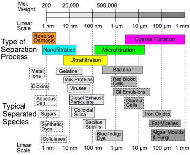
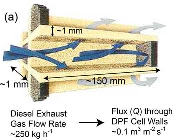
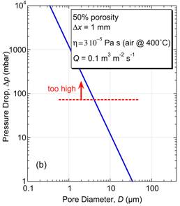
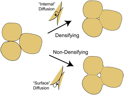
\[{h_i}\Delta T(4\pi {(d/2)^2}) = c\left( {\frac{{{\rm{d}}T}}{{{\rm{d}}t}}} \right)\left( {\frac{4}{3}\pi {{(d/2)}^3}} \right)\]

\[ ∴ \frac{{{\rm{d}}T}}{{{\rm{d}}t}} = \frac{{6{h_i}\Delta T}}{{cd}}\]

If ΔT (initial value) is ~1,000 K, and specific heat, c, is ~3 ×10⁶ J m^-3 K^-1, then the heating rate is ~4 × 10⁷ K s^-1 for a fine particle and ~2 ×10⁴ K s^-1 for a coarse one. These are both high rates, but particle size clearly has a strong effect. With typical flight times of the order of a few tens of ms, even 100 μm particles will become heated, but perhaps only by a few hundred K. For this reason, large particles (>100 μm) are rarely used in thermal spraying and, particularly for materials with high melting points (eg ceramics), it's often necessary for particles to be relatively small (<~50 μm), as well as making the gas temperature as high as possible.

The simulation below, in which these relationships are used to estimate both the particle temperature and its Stokes number on reaching the substrate, allows exploration of the conditions needed to ensure that a deposit is formed (ie that the particles will strike the substrate while molten), for some selected materials.

Passage of particles through filter

Mechanical filtering (trapping particles in some sort of mesh or porous medium) is an obvious method of removing harmful particulate from a fluid (notably both air and water), although it is not really a suitable approach to obtaining or classifying powder fractions. (While it is sometimes possible to clean, or "regenerate", filters, it's not normally practicable to extract powder from them.) Key filtration issues relate to the twin (conflicting) requirements of trapping (fine) particulate, while avoiding substantial inhibition of the fluid flow. The latter may concern clogging, and the possibility of periodic removal of trapped material, but a fine filter, even when clean, may require a relatively high pressure drop across it to create the necessary flow rate.

There is interest in filtration of many species from fluids, ranging from coarse inorganic suspensions to small dissolved ions. This is illustrated in the figure below, which shows some of the terms commonly used to denote different types of filtration and corresponding length scales. Small molecules and ions cannot be removed via mechanical entrapment and require precipitation or osmotic separation. However, provided a suitably fine permeable medium is available, mechanical filtration can be effective for very small species (down to ~1 nm), although this may be at the cost of very low fluid flow rates - see below.

Terms used for filtration

The pressure drop (Δp) across a filter of thickness Δx, needed to generate a fluid flux through it of Q (m3 m‑2 s‑1) is dictated by Darcy’s law

\[Q = \frac{\kappa }{\eta }\frac{{\Delta P}}{{\Delta x}}\]

where η (Pa s) is the viscosity of the fluid and κ (m²) is the specific permeability of the medium (filter). Finer filters do, of course, tend to have lower permeabilities, leading to larger pressure drops and/or lower flow rates. This equation can be used to explore specific filtration requirements. There are expressions available for prediction of the permeability of a porous medium, such as the Carman-Kozeny equation, which is described here.

In the simulation below, a flow situation can be set up in terms of applied pressure gradient (pressure drop and filter thickness), filter type (fibre or particle size and porosity level) and fluid type, both chosen from a small number of options. (The DPF option for filter type is a Diesel Particulate Filter - see the following page.) For each of these, the Carman-Kozeny equation is used to give a permeability, which is then employed to predict the fluid flux (represented as the velocity of markers - there is no depiction of particles becoming trapped in this simulation).

Diesel particulate filters

An important and demanding filtration requirement is that for automotive Diesel engine exhaust, from which very fine (10-100 nm) carbon particles must be removed. Such particulate is present in many combustion exhausts - candle flames are particularly rich in it - and the level in Diesel exhaust is relatively high. The gas flow rate for a Diesel car is ~250 kg h^-1, the exhaust pipe diameter is ~150 mm and a back-pressure above ~100 mbar across the filter would impair operation of the engine. The filter surface area is raised via a honeycomb geometry of the type illustrated below (doi:10.1595/147106709x390977), so that the high flow rate creates only a fairly low flux through the filter wall, Q, of ~0.1 m³ m^-2 s^-1 (ie a gas velocity of ~0.1 m s^-1), and the wall thickness, Δx, is kept low (~1 mm). The Carman-Kozeny equation was used to create the figure below giving the pressure drop as a function of pore size, based on the filter material having the structure of a set of parallel cylinders, with a porosity level of 50%. The plot suggests that pore dimensions finer that a few microns will lead to an unacceptably high pressure drop and in fact DPFs are normally made by lightly sintering together relatively coarse particulate, creating pores with dimensions of tens of microns.

This appears problematic for filtration of substantially sub-micron particles. Fortunately, the carbon particles in Diesel exhaust adhere well to each other, so that a network of them builds up fairly quickly in the pores. When “clean”, however, the filtration efficiency is relatively low, and filters are repeatedly returned to this state, since they need to be “regenerated” every few hundred km (by injecting fuel into the exhaust, so that the accumulated carbon particles are burnt off). This is illustrated in the figure below, which shows experimental data for the pressure drop across a DPF, as a function of mass gain during operation, and the initial filtration efficiency after regeneration.

DPS soot mass

Soot

In practice, there are several factors that influence the choice of material and production route for a DPF, including a need to be resistant to high temperatures and thermal shock. Some details are supplied here.

Powder consolidation by cold pressing and sintering

Powder processing is often an attractive alternative to casting or deformation processing in order to produce shaped components. There are many situations in which it is the only viable option - for example, if the material is difficult to melt, contain or deform. The powder is mixed with some sort of fugitive (usually polymeric) binder and moulded into the required shape, often by simply applying pressure at ambient temperature to a flexible (rubber) mould containing the mixture. The resultant "green compact" is then fired at high temperature (usually well below the melting temperature of the material), when the binder is driven off and the compact becomes consolidated as a result of sintering - see below. The powder may be just a single species, although sometimes "sintering aids" are added.

Sintering often requires extensive diffusion, so the temperature usually needs to be relatively high (>~0.6T_m). The diffusion is driven by the resultant reduction in surface area. On a local scale, diffusion tends to reduce the local curvature of the free surface. This is illustrated in the figure below, where it can be seen that the diffusion can either occur within the surface or can be "internal" - ie through the lattice or via preferred routes such as grain boundaries or dislocations. This figure highlights an important point, which is that, while both types of diffusion cause growth of necks (via transport of material to regions of high surface curvature), raising the strength of the compact, only internal diffusion leads to densification (ie movement of the centres of particles towards each other). It's sometimes desirable to create strong compacts with relatively high porosity levels (eg for lubricated bearings). In such cases, conditions are sought that will favour surface diffusion over internal diffusion.

Internal diffusion leading to neck growth

The animation below shows schematic depictions of the processes of mould filling, cold pressing and the diffusion that causes neck growth (with or without densification). Also shown are representations of the process variants of liquid phase sintering, reactive sintering and hot isostatic pressing (HIP).

Summary

You should now understand at least some of the basic principals involved in processing of powders. This TLP does not cover all aspects of powder technology - for example, there is nothing on production of powders, on their classification into different size ranges or on their safe handling. Nevertheless, much of the underlying science, particularly that governing the dynamics of particles in fluid streams, has been covered here and you should be able to carry out simple calculations concerning sedimentation of powder particles in fluids and on whether they are likely to strike obstacles in a fluid stream - this is relevant, for example, to their removal by filtration and to the process of thermal spraying . The significance of the Reynolds number, the Stokes number, the Biot number, Darcy’s law and the permeability of a porous medium are all described in the context of powder processing. Moreover, the procedures that are commonly used to produce artefacts from metal and ceramic powders are described, although there is no quantification of the sintering phenomena that take place during them.

Questions

Quick questions

You should be able to answer these questions without too much difficulty after studying this TLP. If not, then you should go through it again!

The Reynolds number is a measure of:

The terminal velocity of a particle falling under gravity in a fluid is:

The Stokes number is a measure of:

	a	The ratio of the velocity of a particle in a fluid to the velocity of an obstacle in its path, and hence of the likelihood of it striking the obstacle.
	b	The ratio of the velocity at which a particle in a fluid is approaching an obstacle, to its terminal velocity in the fluid, and hence of the likelihood of it striking the obstacle.
	c	The ratio of the inertial force acting on a particle moving towards an obstacle, to the drag force exerted by the fluid, and hence of the likelihood of it striking the obstacle.
	d	The time needed for a particle to change its direction of motion, relative to that involved in passing an obstacle in its path, and hence of the likelihood of it striking the obstacle.

The (specific) permeability of a porous medium is:

The sintering process that leads to a relatively loose assembly of powder particles being transformed into a material with acceptable strength and stiffness:

Deeper questions

The following questions require some thought and reaching the answer may require you to think beyond the contents of this TLP.

It is proposed that a new type of Diesel Particulate Filter (DPF), with a very high efficiency for extracting fine carbon particles, could be made by creating a bonded assembly of fine alumina fibres (diameter ~0.1 μm). Use the Carman-Kozeny equation to estimate the expected permeability of such a material, assuming that it will be 80% porous. If the maximum gas flux through the DPF is 500 m³ hr^-1, its surface area is ~1 m² and its wall thickness is ~1 mm, estimate the pressure drop across it and comment on whether this value is likely to be acceptable for satisfactory operation of the engine. [The viscosity of the exhaust gas at the temperature concerned is about 3 10^-5 Pa s.]
It is proposed that thermal spraying will be used to create an alumina (MPt. ~2040˚C) coating on a metal artefact, using a combustion torch with a flame temperature of 2300˚C. The alumina powder to be used has an average particle size of about 20 µm and the heat capacity of alumina c, is ~3 10⁶ J m^-3 K^-1. The stand-off distance to be used is 400 mm and the gas velocity is 200 m s^-1. The interfacial heat transfer coefficient under these conditions is estimated to be 10 kW m^-2 s^-1. Assuming that injected particles reach the gas velocity very quickly, estimate their temperature at impact and hence decide whether the spraying process is likely to be successful.

Going further

Books

Ceramic Processing and Sintering, MN Rahaman, Marcel Dekker, New York (2003) ISBN 0-8247-0988-8.
Introduction to the Principles of Ceramic Processing, JS Reed, Wiley, New York (1988) ISBN 0-471-84554-X.

Websites

European Powder Metallurgy Association site: http://www.epma.com/what-is-powder-metallurgy
Wikipedia entry on ceramic engineering: https://en.wikipedia.org/wiki/Ceramic_engineering

Reynolds number

The Reynolds number is given by:

\[{\mathop{\rm Re}\nolimits} = \frac{{\rho uL}}{\eta } = \frac{{uL}}{\nu }\]

where u is the velocity, L is a characteristic distance, η is the viscosity and ρ is the density. (The parameter ν (=η/ρ) is the kinematic viscosity, or momentum diffusivity, which, like all diffusivities, has units of m² s^-1.) The values of u and L usually relate to solid objects (pipes, obstacles etc) in or around the flow. For a particle in a fluid, they would normally be the far-field relative velocity and the particle diameter, d. For powder particles (d ~10-100 μm) in air (η ~ 2 10⁵ Pa s, ρ ~ 1 kg m³, ν ~ 2 10⁵ m² s^-1), the value of Re is likely to be low (<~10), and hence the flow laminar, unless the velocity is quite high (>~10–100 m s^-1).

Stokes law

Stokes law can be written

F_dr = 3 πdηu

where d is the particle size, u is the relative velocity and η is the viscosity of the fluid.

Fraunhofer scattering

Particles interrupt the incident beam, leaving secondary wavelets from surrounding regions to reinforce in certain directions, in a similar way to that observed with a diffraction grating. As in that case, the directions in which this occurs are inclined at greater angles to the incident direction when spacings (particle sizes) are smaller. The scattering angle, θ, is given by

\[\sin \theta = \frac{{1.22\lambda }}{d}\]

where λ is the wavelength and d is the particle size. The scattering angle θ is thus larger for smaller particles.

Stokes number

In a steady state, the particle will be carried at the velocity of the fluid, u, so the time to pass an obstacle of size D is of the order of (D/u). From the relationship between terminal velocity and acceleration, the characteristic time for velocity change is

\[{\tau _{\Delta u}} \approx \frac{{\Delta \rho {d^2}}}{{18\eta }}\]

The Stokes number (ratio of these two times) is thus given by

\[{\rm{Stk}} \approx \frac{{\Delta \rho {d^2}u}}{{18\eta D}}\]

It follows from this expression that fine particles will tend to be carried through without impact, while coarse ones will strike the obstacle (to which they may or may not adhere). This depends, however, on the velocity and viscosity of the fluid, as well as on the density difference and the obstacle size.

The Carman-Kozeny Equation

This is an empirical relationship, usually expressed as

\[\kappa = \frac{{{P^3}}}{{\lambda \left( {1 - P} \right){}^2{S^2}}}\]

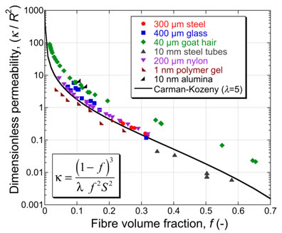
where P is the porosity level, S is the specific surface area (m² m^-3) and λ is a dimensionless constant (typically having a value of ~5). Fine filters tend to have large values of S, leading to low permeabilities. The equation takes no account of the pore architecture (beyond its influence on S). The connectivity of the pores is in practice a key issue. (A material with a high volume fraction of coarse, isolated pores would have a relatively large value of Κ according to the above equation, but would in fact be impermeable - ie Κ = 0.) Nevertheless, the equation is often a useful guide, at least for materials with good pore connectivity, such as fibrous membranes. This is illustrated by the figure below, which is a plot of dimensionless permeability, allowing values to be plotted for membranes of fibres with a wide diameter range.

carman equation

DPF Materials

Clearly, a DPF needs to remove the carbon particulate, without significantly impeding the gas flow. However, there are several further requirements. A major one is stability when subjected to high temperatures, high thermal gradients and thermal shock. This is particularly important during regeneration, which does not occur uniformly and can raise local temperatures to >1000˚C. Even if the phases remain thermodynamically stable, thermal stresses may be high and can cause cracking, ending the life of the DPF (and releasing large amounts of particulate into the atmosphere before it is replaced.) A figure of merit commonly used for thermal shock resistance (TSR) is given by

\[M = \frac{{{G_c}(1 - 2\nu )K}}{{E\alpha }}\]

where G_c is the fracture energy (toughness), n the Poisson ratio, K the thermal conductivity, E the Young’s modulus and α the thermal expansivity. (M has units of power, with a high value reflecting a capacity to withstand high local rates of energy release without cracking.) This equation can be used to identify candidate materials with good TSR and the M values shown in the table below are for materials commonly used for DPFs. It can be seen, for example, that SiC has a high value of M (mainly because of its high thermal conductivity), while Al₂TiO₅ is also attractive (mainly because of its low expansivity and low stiffness). However, the table also highlights an important point, concerning the effect of porosity, illustrated via the example of cordierite (the cheapest of the three materials). The stiffness (E) is often reduced substantially by high levels of porosity, which DPFs require in any event.

Property	Material (fully dense)				Porous Cordierite
Property	SiC	Al₂TiO₅	Al₂O₃	Cordierite	Porous Cordierite
Fracture energy, G_c (J m^-2)	25	20	50	40	15
Young’s modulus, E (GPa)	450	20	300	140	10
Poisson ratio, ν(-)	0.14	~0.2	0.21	~0.2	~0.2
Thermal conductivity, K (W m^-1 K^-1)	120	1.5	18	3	~2
Thermal expansivity, α (K^-1)	4 × 10^-6	1 × 10^-6	8 × 10^-6	2 × 10^-6	1 × 10^-6
Figure of Merit, M (mW)	1.2	0.9	0.2	0.3	1.8

Academic consultant: Bill Clyne (University of Cambridge)
Content development: Arthur Kuenzi
Photography and video: Steve Penney
Web development: Lianne Sallows and David Brook

ThisDoITPoMS TLP was funded by the UK Centre for Materials Education and the Department of Materials Science and Metallurgy, University of Cambridge.

	a	The ratio of inertial forces to viscous forces, and hence of the tendency for fluids to flow faster.
	b	The ratio of inertial forces to viscous forces, and hence of the tendency for fluids to flow more slowly.
	c	The ratio of inertial forces to viscous forces, and hence of the tendency for fluid flow to become chaotic.
	d	The ratio of the speed of a fluid to its dynamic viscosity, and hence of the tendency for fluid flow to become chaotic.

	a	Proportional to the square of its size.
	b	Independent of its shape.
	c	Independent of the fluid viscosity.
	d	Independent of temperature.

	a	The proportionality constant relating the flux of a fluid through the medium to the pressure gradient divided by the fluid viscosity.
	b	Directly proportional to its porosity.
	c	The proportionality constant relating the average velocity of a fluid flowing through the medium to the pressure gradient divided by the fluid viscosity.
	d	Independent of the specific surface area of the medium.

	a	Always involves removal of most or all of the porosity.
	b	Requires the application of imposed pressure at high temperature.
	c	Is driven by reduction of the surface area within the powder assembly.
	d	Involves flow of a liquid and/or chemical reactions.