Creep Deformation of Metals (all content)

Note: DoITPoMS Teaching and Learning Packages are intended to be used interactively at a computer! This print-friendly version of the TLP is provided for convenience, but does not display all the content of the TLP. For example, any video clips and answers to questions are missing. The formatting (page breaks, etc) of the printed version is unpredictable and highly dependent on your browser.

Contents

Main pages

Additional pages

Aims

On completion of this TLP package, you should:

• Have an appreciation of the mechanisms involved in creep deformation, and their general dependence on temperature and stress
• Understand what is meant by Primary, Secondary and Tertiary Creep
• Know how creep curves can be represented by (empirical) constitutive laws, and how the values of parameters in them, such as stress exponents and activation energies, can be obtained from experimental data
• Know how a conventional uniaxial creep test is carried out
• Be familiar with a particular set-up for experimental study of the creep characteristics of a material, available in wire form
• Understand the basics of Indentation Creep Plastometry

Before you start

The following TLPs are relevant and could be consulted before you start:
Mechanical Testing of Metals
Mechanisms of Plasticity
Stress Analysis and Mohr's Circle
Finite Element Method

Introduction

When a material is subjected to a stress that reaches the yield stress, it deforms plastically (permanently). Provided the stress is kept below this level, then in principle it should only deform elastically. However, if the homologous temperature is relatively high (above ~0.4) then in practice plastic deformation can occur, even if the applied stress is lower than the yield stress. This deformation is usually progressive with time and is commonly known as creep.  During loading under a constant stress, the strain tends to vary with time approximately as shown below, where the effect of changing the applied stress is also indicated. The graph below is a plot of creep strain.  The elastic strain has been omitted.  In practice, it is quite common to do this (for plasticity, as well as for creep).  It’s worth noting that elastic strains rarely exceed a small fraction of a %, at least for metals, whereas both plastic strains and creep strains commonly reach the range of several tens of %.

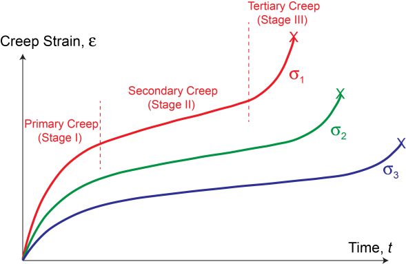
 Schematic creep curves, for 3 different levels of applied stress (σ₁ > σ₂ > σ₃)

The terms “Primary”, “Secondary” and “Tertiary” creep are widely used.  At a simple level, they are often associated respectively with the concepts of: (i) setting up some kind of mechanistic balance, (ii) steady state (constant strain rate) deformation occurring once this balance has been set up and (iii) the breakdown of this balance, often with defects starting to appear and failure rapidly following.

In reality, even without going into details of the mechanisms involved, this picture is simplistic and potentially misleading.  For example, the transition between primary and secondary regimes is often poorly-defined and indeed a true steady state may never be set up.  Furthermore, creep tests are commonly carried out with a constant applied load (rather than a constant true stress). Thus, for tensile tests, the tertiary regime may actually be a consequence of the fact that the true stress is rising throughout the test, with the rate of increase becoming greater towards the end of the test.  At least in some cases, the tertiary regime may be associated with the true stress starting to approach or exceed the yield stress of the material.  The situation can be further complicated by the possibility that significant microstructural changes (such as recrystallization), which could strongly affect the mechanical response, may occur during the test.

These issues are examined in this TLP, together with some details concerning creep mechanisms and the ways in which creep testing can be carried out, and the resultant experimental data interpreted.

Creep Mechanisms

The detailed mechanisms responsible for creep tend to be complex.  However, they almost always involve diffusion of some sort.  This is how the time-dependence arises, since diffusional processes are progressive with time.  Further information about the fundamentals of diffusion is available in the Diffusion TLP.

Creep deformation is caused by the deviatoric (shape changing) component of the stress state applied to a sample – the von Mises stress. The hydrostatic component has no effect, meaning that during creep deformation occurs at constant volume. However, whilst the overall deformation is in response to the deviatoric stress, local variations in in hydrostatic stress do affect creep behaviour, as will be outlined below.

Coble Creep

Creep deformation often involves various defects, particularly dislocation cores or grain boundaries.  These may simply act as fast diffusion paths, or play a larger role in creep mechanisms (some of which are beyond the scope of this TLP), depending on factors such as dislocation density, grain size, grain shape and temperature.   The shape change experienced by the sample may arise simply from atoms becoming redistributed by diffusion.  When this occurs on the scale of a grain, with the diffusion occurring mainly via grain boundaries, then this is commonly referred to as Coble Creep.  The simulation below shows how this tends to cause the sample to extend under an applied load.

Note: Coloured atoms are no different from those in the bulk, but merely allow each atom to be identified easily.

Simulation demonstrating Coble creep on the atomic scale

It can be seen that raising the applied stress accelerates the rate of deformation.  The driving force for this net migration of material (from the “equatorial” regions of grains to the “polar” regions) is that an applied tensile stress like this creates hydrostatic compression in the equatorial regions and hydrostatic tension in the polar regions.  The hydrostatic tension can be thought of as arising from the applied tensile stress, where the compression arises from the lateral contraction of the sample (due to volume conservation). The atoms then tend to move from the more “crowded” to the more “open” regions.  The diffusive flux can be considered as a migration of vacancies in the opposite direction to the motion of atoms, although the concept of vacant sites is less well-defined in a grain boundary than in the lattice.  We could equally imagine how hydrostatic compression could arise in the “polar” regions, and hydrostatic tension could arise in the “equatorial” regions, via the application of a compressive stress to the sample. Hence diffusive flux would be in the opposite direction, and the sample would deform in the opposite fashion, with the grains becoming “squashed” by the compressive stress.

It’s also clear that raising the temperature increases the creep rate.  This is simply due to the rates of diffusion becoming higher as a consequence of the Arrhenius dependence (click here for details).  The activation energy for grain boundary diffusion is low, and the cross-sectional area available for diffusion along grain boundaries is much less than for diffusion through the bulk. Therefore this type of creep is often the dominant one at relatively low temperatures and for samples with a fine grain size.

Nabarro-Herring Creep

A similar type of creep deformation to that described above can occur with the diffusion being predominantly within the interior (crystal lattice) of the grains, rather than in the grain boundaries.  This is often termed Nabarro-Herring creep (N-H creep).  It is depicted in the simulation below.

Simulation demonstrating Nabarro-Herring creep on the atomic scale

A similar dependence on temperature and stress is observed to that for Coble creep.  The diffusion of atoms in one direction can be more easily pictured as the diffusion of vacancies in the other direction during N-H creep. There is a considerably greater sectional area available via crystal lattice paths, particularly if the grains are relatively large.  On the other hand, the activation energy is higher, so diffusion rates tend to be low, particularly at low temperature.  This type of creep tends to dominate over Coble creep at relatively high temperature, and with large grains or single crystals.

Dislocation Creep

Purely diffusional creep (Coble and Nabarro-Herring) is fairly simple, and does occur under certain conditions  -  usually with relatively low applied stresses.  With higher stresses, it is common for a type of creep to occur that involves motion of dislocations, particularly in metals, where dislocation densities tend to be high.  Provided the stress is below the yield stress, conventional macroscopic plasticity, occurring predominantly via dislocation glide, should not occur.  However, with stresses that are starting to approach the yield stress, and are maintained for extended periods, progressive dislocation motion, and hence macroscopic plastic deformation, can occur, often facilitated by extensive climb (absorption or emission of vacancies at the core) of individual dislocations. It should be noted that climb does not refer only to vertical motion of the dislocation, and can refer to horizontal motion too.  One of the ways dislocation creep can occur via climb is shown in the simulation below:

Simulation demonstrating Dislocation Creep on the atomic scale

In this example, the shear stress provides the driving force for diffusion into the dislocation core, rather than hydrostatic compression or tension as in the case of Coble or N-H creep. In detail, there are several different ways in which combinations of dislocation glide and diffusion in the vicinity of dislocations can promote creep.  Some of these have been given specific names, but these often relate to observed dependences on the main variables (e.g. temperature or grain size), rather than being clear about the precise mechanisms involved.  In general, they all involve some combination of dislocation climb and glide, although, in particular cases, factors such as the presence of obstacles (e.g. fine precipitates), the ease of cross-slip etc. may affect the observed behaviour. Dislocation density may also affect the behaviour. However, at the high homologous temperatures at which creep typically occurs, the dislocation density may decrease somewhat with time, or could indeed drop sharply if recrystallization were to occur. It might be imagined that this would reduce the rate of deformation. However, in practice the associated decrease in the yield stress might well promote the onset of conventional plasticity - ie extensive dislocation glide - such that the rate of deformation increased.

Constitutive Laws for Creep

Effects of Microstructure on Creep

As with plastic deformation, creep is a complex process that is strongly affected by the microstructure of the material.  (Some of the microstructural effects that influence plasticity are summarised in the TLP on Mechanical Testing.)  As with plasticity, however, guidelines can be identified concerning features likely to affect (inhibit) creep, and some of these are similar for the two.  For example, a fine array of precipitates, which will inhibit dislocation glide and hence raise the yield stress, is also likely to inhibit (dislocation) creep.  However, there are limits to such linkage.  For example, precipitates might dissolve at the high temperatures involved in creep.  More fundamentally, some features can affect creep and plasticity quite differently.  For example, while a fine grain size tends to raise the yield stress, as a result of grain boundaries acting as obstacles to dislocation glide, it can cause accelerated creep in a diffusion-dominated regime, since such boundaries also constitute fast diffusion paths.

Nevertheless, as with plasticity, empirical constitutive laws can be used to model and predict creep behaviour.  There is sometimes scope for interpreting the values of parameters in these laws in terms of the dominant mechanisms involved.  In particular, if rates of creep are measured over a range of temperature, then it may be possible to evaluate the activation energy, Q (in an Arrhenius expression), which could in turn provide information about the type of diffusional process that is rate-determining.  It is also often claimed that the value of a stress exponent, n, obtained via creep rate measurements over a range of applied stress, is indicative of the dominant mechanism, with a low value (~1-2) indicating pure diffusional creep and a higher value (~3-6) suggestive of dislocation creep.  The theoretical basis for such conclusions may sometimes be questioned, and in any event these laws must be recognised as essentially empirical, but it is certainly important to be able to characterize the creep response of a material, and to be clear about the regime of temperature and stress for which a particular law is valid.

General (Steady State) Creep Law

The creep strain rate (rate of change of the von Mises plastic strain) in the steady state (Stage II) regime is often written

\[\dot \varepsilon = A \sigma^n \exp ( - Q/RT)\;\;\;\;\;\;\;\;(1)\]

where A is a constant, σ is the applied (von Mises  -  click here for definition) stress, Q is the activation energy and n is the stress exponent.  This is a relatively simple equation, but several caveats should be added.  The most important of these are apparent in Fig.1 of the Introduction page   -  ie it relates only to the steady state (secondary) regime.  It is sometimes stated that the overall creep life is often dominated by this regime.  In practice, this may or may not be true.  In particular, it’s worth noting that, not only can the primary regime extend over a significant fraction of the creep lifetime, but also, since the creep rate is often much higher during primary creep, its contribution to the overall creep strain can be substantial, and even dominant.  Depending on a number of factors, simply ignoring primary creep may be highly inappropriate.

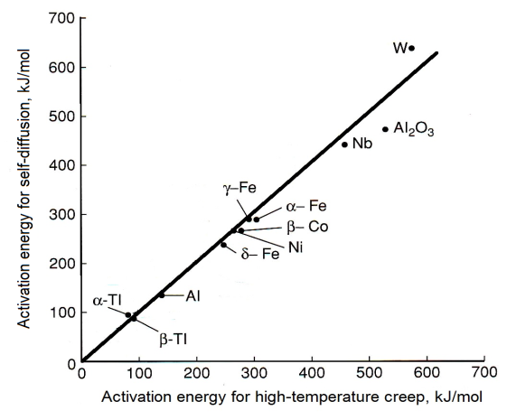
Plot of self-diffusion activation energy vs. high temperature creep activation energy, with a line drawn along which the two are equal. [1]

It may be noted that the activation energy for creep at high temperatures is often found to agree closely with that for bulk diffusion  -  see, for example, the data in the figure.  This is consistent with the concept of N-H creep (diffusion through the lattice) dominating Coble Creep (grain boundary diffusion) at high temperatures.

Laws Capturing both Primary and Secondary Regimes

In view of the potential importance of the primary regime, there is strong interest in using modelling approaches that incorporate it.   Several expressions have been proposed for capture of both primary and secondary regimes, and of the transition between them.  One that can be taken as representative is the following equation, which is sometimes termed the Miller-Norton law

\[{\varepsilon _{{\rm{cr}}}} = \frac{{C{\sigma ^n}{t^{m + 1}}}}{{m + 1}}\exp \left( {\frac{{ - Q}}{{RT}}} \right) \;\;\;\;\;\;\;\;(2) \]

In this expression, C is a constant (units of Pa⁻ⁿ s^−(m+1)), t is the time (s), n is the stress exponent and m is a dimensionless constant.  The simulation below, in which this equation is plotted, can be used to explore Miller-Norton creep strain plots as the 6 parameters involved are varied.

Simulation showing behaviour predicted by M-N law with constant true stress

A number of features should quickly become apparent, such as the high sensitivity to temperature and that the sensitivity to the applied stress increases as the value of n is raised. 

One issue here is whether the applied stress is a nominal or a true value.  It certainly should be a true value, as this is implicit in the M-N law.  However, it is common during testing to fix the load (often in the form of a dead weight), rather than the true stress.  Also, most uniaxial creep tests tend to be carried out in tension.  Neglecting any inhomogeneity that might arise, such as a necking effect - which is not common during creep testing - the true stress will rise as straining occurs and the cross-sectional area reduces.  Depending on the value of n, this could have the effect of causing the strain rate to rise (whereas it would otherwise be falling and approaching a constant value).

This effect is modelled in the simulation below.  The M-N law can be differentiated with respect to time, to give

\[{\dot \varepsilon _{{\rm{cr}}}} = C{\sigma ^n}{t^m}\exp \left( {\frac{{ - Q}}{{RT}}} \right) \;\;\;\;\;\;\;\;(3)\]

Therefore, by stepping in time and repeatedly re-evaluating the true stress, and hence the strain rate, the full creep strain curve can be built up (although it can no longer be expressed as a single analytical equation).  In order to implement this, the relationship between true and nominal stresses is needed:

\[{\sigma _T } = \frac{F}{A} = \frac{{FL}}{{{A_0}{L_0}}} = \frac{{F({L_0} + {\varepsilon _N}{L_0})}}{{{A_0}{L_0}}} = \frac{F}{{{A_0}}}(1 + {\varepsilon _N}) = {\sigma _N}(1 + {\varepsilon _N})\;\;\;\;\;\;\;(4)\]

and also that between true and nominal strains

\[{\varepsilon _T } = \int_{{L_0}}^L {\frac{{{\rm{d}}L}}{L}} = \ln \left( {\frac{L}{{{L_0}}}} \right) = \ln (1 + {\varepsilon _N}) \;\;\;\;\;\;\;(5) \]

The above plot can therefore be modified using Eqns. (3), (4) and (5), with the nominal stress taken as constant.  This is done by stepping forward in small increments of time (ie this is a numerical procedure, rather than just the plotting of an analytical equation).  The sequence is as follows.  After an initial small time increment, true stress and true strain are taken to be equal to the nominal values.  For the next increment, the strain rate is obtained using Eqn.(3), and hence the increment of (true) strain obtained on multiplying this by the time increment.  In order to use Eqn.(3), the true stress is needed.  This is obtained using Eqn.(4), with the nominal strain obtained from the true strain using Eqn.(5).  This operation is repeated after every time step, with the true stress progressively rising.

In the simulation below, the stress selected is a nominal value. Depending on several factors (particularly the value of n), a significant rise in the creep strain rate can be seen. This is sometimes (mis-)interpreted as a “Tertiary” regime, although a similar increase could also arise as a result of microstructural changes (e.g. cavitation).  In the case of uniaxial compressive testing, the strain rate will tend to fall, due to a drop in true stress, and hence no such regime will be seen. Of course, these effects will only be noticeable at relatively high strains (say, >~10%), although in practice these are common during uniaxial creep testing.

This figure compares the (tensile) creep strain plot of the standard M-N equation, using a constant nominal stress, with that obtained by stepping through time, repeatedly evaluating the true stress and then using that in the differential form of the equation

It should also be noted that this analysis is based on the Miller-Norton equation being valid, over the range of stresses being considered.  In fact, if the stress rises significantly, then this may not be the case.  In particular, if the true stress starts to reach the yield stress, then conventional plasticity may be stimulated, which would probably be apparent in a creep strain plot as a sharply increasing strain rate.  In fact, this may be responsible for much observed “Tertiary Creep”, rather than it being an effect that can be fully captured by applying the Miller-Norton equation while taking account of the changing true stress.

[1] https://www.intechopen.com/books/superalloys/phase-equilibrium-evolution-in-single-crystal-ni-based-superalloys

Uniaxial Creep Testing - Practical Basics

Many of the practical issues outlined in the TLP on Mechanical Testing (for Plasticity) apply equally to Creep Testing.  For tensile testing, the gauge length must have a smaller sectional area than the region that is gripped, such that the latter undergoes only elastic deformation.  This is not the case for compressive testing, where the sample usually has a uniform section along its length, and is located between hard platens.  For Creep Testing, however, there are additional challenges.  For example, it is commonly carried out at high temperature, so a furnace (with good thermal stability) is needed, and all of the sample must be held at the selected temperature.  Also, the load must be sustained for long periods  -  perhaps just a few hours, but in some cases periods of many weeks or even many months might be needed.  Such conditions bring slightly different challenges from those of conventional (stress-strain) testing.

Nominal or True Levels of Stress and Strain?

As for conventional testing, there is the issue of true or nominal versions of both stresses and strains.  However, there is a difference with Creep Testing.  For Stress-Strain Testing, the applied load is being ramped up continuously, so the issue reduces to that of converting any particular load level to a stress in the sample.  Provided the stress is uniform throughout the sample, a simple equation can be used to convert an applied load to a true stress.  A similar operation allows an extension (nominal strain) to be converted to a true strain.   There is a rather more fundamental problem with Creep Testing.  As noted in the Introduction page of this TLP, creep is characterised by a series of strain-time curves for different levels of (true) stress.  Under fixed load conditions, the true stress changes continuously during the test, so these curves will be unreliable (for tests in which relatively large strains are generated).

Fixed Load Machines

Many creep facilities are based on a fixed load, applied via a dead weight (with a lever arrangement such that the actual applied force is considerably larger than the weight itself).  A typical facility of this type is shown below.  The actual weight used is unlikely to be much more than a few tens of kg.  However, with the lever arm arrangement giving a mechanical advantage of at least 10, and perhaps considerably more, such weights can produce an applied force on the sample of up to several tens of kN.  This is usually sufficient for most situations (sample dimensions and required stress levels), although the limitations associated with having a fixed nominal stress (varying true stress) should be noted. 

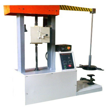
A typical (dead weight) creep frame (produced by Medilab Enterprises)

Variable Load Machines

It is, of course, possible to have a loading frame in which the force (usually produced either by screw-driven or hydraulic systems) can be varied during the test.   A typical facility of this type is shown below.  Such machines can readily generate forces of up to hundreds of kN.  With the strain (extension) being continuously monitored, software control can be used to change the applied load such that a true stress is maintained. However, it is worth noting that such machines tend to be expensive.  They’re not well-suited to very long term tests, both because of potential wear on the loading system and because tying up such expensive facilities for long periods is not economically attractive.  If a number of samples are to be tested over periods of weeks or months, which is not unusual for creep testing, then it is much more likely that a set of dead weight machines will be used.

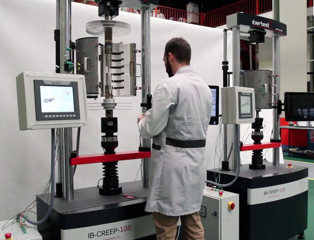
A typical (variable load) creep loading frame (produced by IBERTEST)

Multiaxial Creep Testing – The Creeping Coil

Background

Note: this experiment deals with torsion which can be explored further in the Bending and Torsion of Beams TLP here

This experiment is a simple and convenient one to carry out.  The sample is in the form of a wire that is wound into a coil, which creeps under its own weight.  Using a low melting point material such as lead or solder, this occurs at relatively low temperatures (without heating, or using a simple hot air system).  Several simplifying assumptions are made in carrying out the analysis.  Each turn of the coil is taken to experience a constant stress  -  the average value acting throughout the section of the wire.  Furthermore, it is assumed that the steady state regime of behaviour is immediately established everywhere  -  ie primary creep is neglected.  These are crude assumptions and the experiment cannot be used to obtain quantitative creep characteristics.  However, it is possible to obtain fairly reliable indications of the dependence of creep rates on temperature (ie values of Q) and, to some extent, on stress (ie values of n)

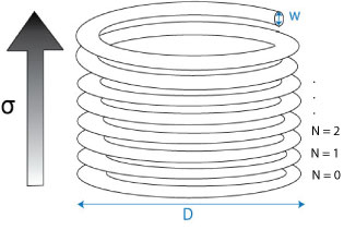
Diagram showing the coil with each turn assigned a number starting from N=0 when the stress is zero

The stress in a particular turn is proportional to its number, N, where the turns are numbered beginning from zero at the bottom turn and ending at the top. The shear stress in each turn varies from zero at the centre of the turning to a maximum value at the edge of the coil and it’s average, τ, is given by:

\[\tau = BN\]

(Derivation)

where B is a constant of proportionality (for this experiment). The coil is then allowed to creep over a fixed amount of time (e.g. one minute) and at the end of this time the spacings, s, between the turns are measured.The average local shear strain γ in each turn is a function of s and is given by

\[\gamma = Cs\]

(Derivation)

where C is a constant. Assuming that steady state creep dominates, the strain rate is simply the strain divided by the time.  This equation can now be used to explore the relationship between strain rate and shear stress

\[\dot \gamma = C\frac{s}{t}\]

Using the steady state creep equation:

\[\dot \gamma = A{\tau ^n}exp\left( { - \frac{Q}{{RT}}} \right)\]

Taking natural logarithms:

\[\ln \dot \gamma = \ln (A) + n\ln (\tau ) - \frac{Q}{{RT}}\]

 using the expressions for average shear stress and average strain rate:

\[ \ln \left( {\frac{s}{t}} \right) =K + n\ln (N) - \frac{Q}{{RT}}\;\;\;\;\;\;\; (*) \]  

where  \(K =\ ln(A) + n\ln(B) - \ln(C)\). This equation can be used to evaluate the creep parameters from (plots of) experimental data.

Experimental Set-Up

In order to create a temperature-controlled environment, the coil is placed inside a Perspex tube. Once the temperature in the tube has stabilised, the coil is allowed to creep under its own weight for one minute. The videos above show qualitatively how creep rate varies with temperature.

Evaluating Parameters

The spacings between the turns of the coil can be obtained from photos or more simply by just rotating the support cylinder until it is horizontal (so that creep will stop).  Spacings are then readily measured directly with a ruler. The spacing of the Nth turn is taken as the distance between the Nth and (N-1)th turn, i.e. the spacing of the 1st turn is the distance between the 0th and 1st turn.  Using the equation above marked with an asterisk, a plot can be constructed of ln(s/t against ln N), at a given temperature, with the stress exponent, n, obtainable from the gradient. A similar operation can be carried out using data for a number of different temperatures, with ln(s/t) plotted against 1/T, for a selected value of N, to obtain the activation energy, Q

Multiaxial Creep Testing – Indentation Creep Plastometry

Indentation creep plastometry is an fairly novel procedure involving use of an indenter, as opposed to conventional uniaxial testing machines.  The process has similarities to indentation plastometry, described in the Mechanical Testing TLP.  The advantages noted there, arising from the procedure being non-destructive, applicable to small samples of simple shape and offering scope for mapping of properties across a surface, also apply here.  Furthermore, while uniaxial creep testing requires a series of tests at different stress levels (and experimental difficulties in maintaining a constant true stress), a single indentation creep experiment allows full characterisation of the creep behaviour (as captured in a constitutive law).

Method

Recess Creation

A spherical indenter is normally used.  As with conventional creep testing, it is important to avoid conventional (time independent) plastic deformation.  This is particularly an issue in the initial stages, when the contact area would be very low as the indenter penetrated a flat surface, and the stresses correspondingly high.  In order to avoid this problem, a (spherical) recess is first created in the sample, matching the indenter.  This procedure can be used to ensure that the stresses in the sample never reach the yield stress (at the temperature concerned).

Test Procedure

The selected load is quickly applied and the penetration recorded as a function of time.  As with Indentation Plastometry, the core of the procedure is iterative numerical simulation of the test, using the FEM method. A constitutive creep relationship, such as the M-N law, is used in the model, with trial, and then improved, values of the (three) parameters in it, with the goodness of fit parameter (S) between predicted and measured displacement-time curves being used to guide the optimisation.  The simulation below shows the outcome of this operation for a particular case (a Ni sample at 750°C, with a 1 kN load, an indenter radius of 2 mm and an initial recess depth of 1 mm, with a 2 mm radius of curvature).  The evolving von Mises stress and strain fields are shown, together with measured and modelled displacement-time plots, with the optimised M-N parameter set

Predicted and mesured curves agree quite well  -  the value of S is 10^-3.2, which is acceptably close to zero.  The parameter set that gave this level of agreement is shown below:

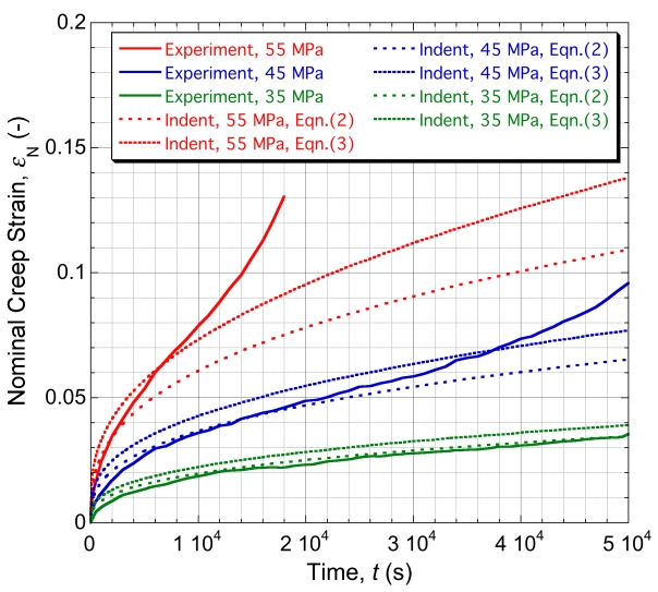
Graph showing how our predictions compare with the experimental data for uniaxial tensile creep testing

Using this parameter set, a prediction can be made (using the M-N law directly, with no need for FEM simulation), of the outcome of uniaxial testing, with any particular applied stress level. The outcome of such operations is compared with experimental data, for this material and test temperature, in the plot shown here. Two sets of predicted plots are shown for each stress level. The first set corresponds to use of Eqn.(2) on the page "Constitutive Laws for Creep" - ie the standard M-N law. In fact, the experimental data were obtained during testing with a fixed load (constant nominal stress), so the appropriate plots are really those marked in the figure as referring to Eqn.(3), which were obtained using the differential form of the M-N law - ie Eqn.(3) on the page "Constitutive Laws for Creep". It can be seen that the agreement with these plots is good, apart from periods towards the end of the test with the higher applied stress levels, when tertiary” behaviour is seen, probably because the true stress was approaching the yield stress (~65 MPa), so that “plasticity” was stimulated.

Designing for Creep Resistance - Nickel Based Superalloys

With over 100,000 flights a day, jet engines are commonplace in today’s world. Jet engines work more efficiently at higher temperatures.  Turbine entry temperatures can be of the order of 1,500°C and, while cooling channels and Thermal Barrier Coatings ensure that the blades do not reach these temperatures, they may be at around 1,000°C -  a temperature at which most metals are likely to undergo rapid creep under the stresses concerned (~100 MPa). The gradual deformation of these blades is not only financially costly, as they will have to be replaced, but could lead to catastrophic failure and hence, in some cases, loss of life. This is why it’s important to understand the creep behaviour of the materials we use and moreover how we can produce materials with improved creep resistance. Diffusion and dislocation motion are the main mechanisms by which the creep of materials occurs and as such limiting them is key to designing creep resistant materials. Jet engine blades are made from Nickel-based superalloys.  A brief outline is presented here of how they are designed, given that resistance to creep at very high temperatures is a key requirement.

Limiting Diffusion

1.Homologous temperature

The (substitutional) diffusivity of a material depends on how easily atoms move between vacant sites in the lattice (see more here), and on the vacancy concentration.  Both jump rates and vacancy concentrations are higher at higher temperatures, approaching limiting values close to the melting temperature.  It is thus the homologous temperature (T/T_m) that is important.  For example, diffusion (and hence creep) rates are relatively high at room temperature for Pb (T/T_m ~0.5), but negligible for Ni (T/T_m <0.2). There are clearly advantages in using materials with high melting temperatures.”

2.Grain structure

There are two important points to be made regarding grains. Firstly, grain boundaries themselves are detrimental to creep resistance because they provide fast diffusion paths through the material and thus accelerate (Coble) creep.  Secondly, the length of a grain in the direction of applied stress dictates the distance an atom must diffuse in order to reach the “polar” regions from the “equatorial” regions. Elongating the grains parallel to the applied stress direction will thus tend to reduce the creep rate.  The latter effect can be obtained with a columnar grain structure, which is relatively easy to create using controlled directional solidification.  Even better is a single crystal (with a selected crystallographic orientation).  This requires somewhat greater control during the casting process, although it can be done and this is now routine for many types of blade.  The figure below illustrates this.

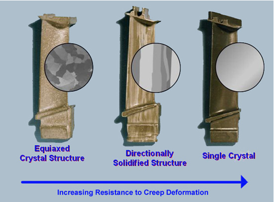
Progression in manufacture of creep-resistant microstructure over time

3.Crystal Structure

In addition to the homologous temperature, there are other factors that can affect the diffusivity.  These include the crystal structure, which dictates both the packing density and the nature of the paths taken during atomic jumps between vacant sites.  In general, diffusive jumps are more difficult in close-packed, high-symmetry structures, such as fcc.  There are also additional factors related to crystal structure.  For example, diffusion is difficult in ordered structures, since diffusion tends to create disorder (that is thermodynamically opposed).  The microstructure of Ni-based superalloys is typically a 2-phase one, composed of an intimate mixture of γ (fcc Ni) and γ’ (an ordered structure based on Ni with Al and/or Ti), with coherent or semi-coherent interfaces between them.  These structures are illustrated below.

Limiting Dislocation Motion

While the two are often inter-related during creep, it is important to inhibit dislocation motion, as well as diffusion.  This happens in several ways in Ni-superalloys.  One of these concerns the ordered γ’ phase.  An ordered structure is degraded, not only by diffusion, but also by dislocation glide.  Such motion is therefore opposed, an effect often described as order hardening.  (In fact, if dislocations move in pairs, sometimes termed superdislocation pairs, then the second of the pair may restore the order, but this does impose a constraint on the motion  -  see below.)  There is also an effect of the coherency of the γ /γ’ interface, which creates lattice strain in the vicinity.  This also tends to inhibit dislocation glide.

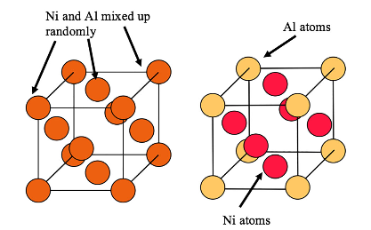
Unit cell of γ on the left and that of γ’ on the right [2]

Precipitates of γ’ exist within a γ matrix, and so dislocations will have to pass from γ to γ’ in order to move through the alloy. The shortest Burgers vector in γ is (a/2)<110>, but in γ’ this is not a lattice vector. As a dislocation passes from γ to γ’ its Burgers vector must be maintained and it will create a region with unfavourable bonding (an anti-phase boundary) and hence an associated energy cost. Its motion is therefore slowed considerably in γ’ compared to that in γ, and it can only travel at any appreciable rate through γ’ once another dislocation passes into γ which restores the unfavourable bonding back to its ordered state – as they move through together the anti-phase boundary maintains a constant width and there is thus no added cost to their motion through γ’. This can be seen in the micrograph below:

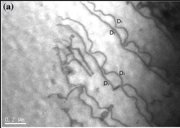
Micrograph showing dislocations passing through a Ni superalloy [3]

It can be seen that dislocations D₁ are impeded by γ’ precipitates with D₂ following unimpeded. This mechanism results in much slower dislocation glide through the alloy as a whole and so is effective in reducing the rate of dislocation creep. The finer the dispersion of γ’ precipitates the more effective the strengthening will be. The two dislocations that pass through γ’ together are called super-partial dislocations and the sum of their burgers vectors is a lattice vector - a<110> - in the γ’ phase. It is important to note that the γ - γ’ interface is coherent and therefore coarsening does not occur over time.

[2]  Y. M. Wang-Koh (2017) Understanding the yield behaviour of L12-ordered alloys, Materials Science and Technology, 33:8, 934-943, DOI: 10.1080/02670836.2016.1215961
[3] Lv, X., Sun, F., Tong, J. et al. J. of Materi Eng and Perform (2015) 24: 143. https://doi.org/10.1007/s11665-014-1307-y

Summary

This TLP covers the mechanisms involved in creep deformation, how it can be modelled and how it can be investigated experimentally. There is also coverage of the need for creep-resistant materials and how they can be designed.

Firstly, the fundamental mechanisms of creep are covered, including the dependence of each on levels of stress and (homologous) temperature.  The key role of diffusion is emphasized, leading to a dependence on time that is not exhibited by conventional plastic deformation.

Secondly, the concept of (empirical) constitutive laws to characterize creep was introduced.  The emphasis is often on Stage II (steady state) creep, but in practice the primary regime often constitutes an important part of the overall behaviour and a law is presented that covers both regimes.  Mention is also made of the so-called tertiary regime (immediately before final rupture), and the possible ways in which it can arise.

Thirdly, there are descriptions of the experimental procedures that can be used to obtain creep characteristics.  The most common of these are the conventional uniaxial (tensile or compressive) tests, which need to be carried out with a series of different applied stresses in order to obtain the values of parameters in constitutive laws.  These procedures are rather cumbersome and time consuming.  It is also shown that test procedures exist in which the stress and strain fields are more complex, but can be analysed – either using a set of equations or via Finite Element Modelling.  The creeping coil experiment and the Indentation Creep Plastometry procedures are described as examples of these, the latter having the potential to at least partly replace conventional creep testing.

Finally, the importance of creep resistance in technological applications was illustrated using the well-known example of Ni-based superalloys in turbine blades for aero-engines and power generation plants.  The microstructure of these components, and the ways in which their design and production have been approached, are related to the optimisation of creep resistance, based on various principles outlined earlier in the TLP.

Questions

Quick questions

You should be able to answer these questions without too much difficulty after studying this TLP. If not, then you should go through it again!

1. Which of the following could be reasons tertiary creep is observed?

   	a	Rising true stress can cause the strain rate to rise
   	b	Microstructural damage such as cavitation can occur
   	c	Rising true stress can exceed the yield stress, causing conventional plastic deformation
   	d	All of these"

2. In the γ/γ' structure of Ni-based superalloys, why is the existence of a coherent interface important?

   	a	It leads to lattice strains that can inhibit dislocation motion
   	b	The ordered structure of the γ' phase inhibits diffusion
   	c	The ordered structure of the γ' phase inhibits dislocation motion
   	d	All of these

3. What is the function of the recess in Indentation Creep Plastometry?

   	a	It prevents tertiary creep
   	b	It allows the stresses created during the early stages of the process to be kept relatively low (below the yield stress)
   	c	It ensures that the indenter is located properly before indentation starts
   	d	It removes the near-surface region, which could have different properties from the bulk
   	e	It eliminates primary creep, so that the steady state regime is immediately established

Deeper questions

The following questions require some thought and reaching the answer may require you to think beyond the contents of this TLP.

4. Why is creep deformation different from conventional deformation?

   	a	Strain develops at a much slower rate in the material
   	b	Strain produced depends on the time for which the stress is applied
   	c	Creep cannot occur at room temperature
   	d	The strain produced doesn’t depend on the applied stress

5. Which of the following statements is true?

   	a	Only Coble creep is controlled by diffusion
   	b	Only Nabarro-Herring creep is controlled by diffusion
   	c	Only dislocation creep is controlled by diffusion
   	d	All of the above mechanisms are controlled by diffusion

6. Which of the following is not an assumption that we make during the creeping coil experiment?

   	a	Assume constant true stress when we have constant load
   	b	Assume that the stress is uniform throughout each turn
   	c	Assume that only steady state creep occurs throughout
   	d	Assume that the creep regime is the same throughout the coil

7. Which of the following features of Ni superalloy turbine blades helps to make them resistant to creep? (There may be more than one)

   Yes	No	a	Fine grain structure
   Yes	No	b	Single crystal
   Yes	No	c	High dislocation density
   Yes	No	d	High purity
   Yes	No	e	Order hardening due to γ' precipitates in γ matrix
   Yes	No	f	Low inherent diffusivity of FCC structure

Going further

There are many publications covering creep, over a wide range of depths. Some go into much greater detail than this TLP. The following books
provide a good overview:

Books

Fundamentals of Creep in Metals and Alloys, Michael Kassner, Butterworth-Heinemann, 2015, ISBN: 9780080994277

Creep of Metals and Alloys, RW Evans & B Wilshire, CRC Press, 1985, ISBN-10: 0904357597"

Regarding Indentation Creep Plastometry, which is a very recent development, there are as yet no published books and indeed the software necessary to implement the technology is not yet widely available in user-friendly, commercially mature form.  However, there are websites that describe the methodology, where such access is likely to become available in due course.  Notable among these is https://www.plastometrex.com/.

Derivation of τ

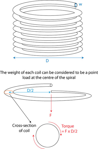
F = total weight of coil below turn = volume x density x acceleration due to gravity

\[F = \left( {\frac{{\pi {w^2}}}{4} \times \pi D \times N} \right) \times \rho \times g\]

T = Torque = \(\left( {\frac{{\pi {w^2}}}{4} \times \frac{{\pi {D^2}}}{2} \times N} \right)\)\( \times \rho \times g\)

The equation for the shear stress caused by torsion is,\(\tau = \) \( \frac{{Tr}}{J} = \frac{{Tr}}{{2I}} \)

where r is the radial distance from the centre of the wire (\(0 \le r \le \frac{w}{2}\)) and J is the polar moment of inertia (m⁴) which, in the case of a circular cross section, is equal to twice I, the second moment of area ( = \(\frac{{\pi {w^4}}}{{64}}\))

Therefore the shear stress varies from zero at the centre of the wire to a maximum value at its surface:

\[{\tau _{_{\max }}} = \frac{{16T}}{{\pi {w^3}}} = 2\pi \rho g{D^2}\frac{N}{w}\]

An important note is that the average shear stress, τ, is proportional to the peak shear stress:

\[\tau \propto \frac{{N{D^2}}}{w}\]

Furthermore, by noting that D and w are control variables in our experiment we can simplify our expression to:

\[\tau = BN\]

where B is a constant for this experiment

Homologous Temperature

The diffusivity of a material depends on how easily atoms can move to a vacant site on the crystal lattice (see more here). This becomes easier near the material’s melting point and hence it is the materials temperature relative to its own melting point (T_m) – its homologous temperature (T/T_m) – that influences its diffusivity. Rates of N-H creep and dislocation creep are both controlled by bulk diffusion and hence reduced when the diffusivity of a material is lower. The importance of the idea that it is homologous, not absolute temperature, which controls creep rate in the creeping coil experiment, in which lead undergoes easily perceptible deformation via creep at room temperature - 300K represents a significant homologous temperature of ~0.5 for Lead, but an insignificant ~0.2 for Nickel.

Constant True Stress

Is the applied stress a nominal or a true value.  It certainly should be a true value, as this is implicit in the M-N law.  However, it is common during testing to fix the load (often in the form of a dead weight), rather than the true stress.  Also, most uniaxial creep tests tend to be carried out in tension.  Neglecting any inhomogeneity that might arise, such as a necking effect - which is not common during creep testing - the true stress will rise as straining occurs and the cross-sectional area reduces.  For all values of n, this will cause the strain rate to rise, whereas it would otherwise be falling and approaching a constant value.

Derivation of γ

This small element of the wire subtends an angle dβ at the centre of the coil.

The shear strain produced by torsion is given by

\[\gamma = \frac{{{\rm{distance\; through\; which\; we\; twist}}}}{{{\rm{distance\; over\; which\; twist\; occurs}}}}\]

Which can be simplified, algebraically, to

\[\gamma = \frac{r}{2}{\theta _L}\]

where θ_L is the angular twist per unit length induced by the torque and r is the radial distance from the centre (\(0 \le r \le \frac{w}{2}\)).

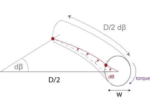
The torque acting on this element causes it to twist through an angle dθ.

Therefore, the twist per unit length is:

\[{\theta _{\rm{L}}} = \frac{{{\rm{d}}\theta }}{{(D/2){\rm{d}}\beta }}\]

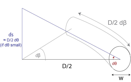
The vertical deflection of the coil due to the twisting of this element is:

\[{\rm{d}}s = \frac{D}{2}{\rm{d}}\theta = {\left( {\frac{D}{2}} \right)^2}{\theta _{\rm{L}}}{\rm{d}}\beta \]

The vertical deflection associated with the twist in one turn of the coil is:

\[s = \int_0^{2\pi } {{{\left( {\frac{D}{2}} \right)}^2}{\theta _{\rm{L}}}{\rm{d}}\beta = \frac{{\pi {D^2}}}{2}{\theta _{\rm{L}}}} \]

The peak local shear strain is thus given by:

\[{\gamma _{{\rm{max}}}} = \frac{{sw}}{{\pi {D^2}}}\]

It may be noted that the average local shear strain, γ, is proportional to the peak strain,

\[\gamma \propto \frac{{sw}}{{ {D^2}}}\]

As we did for the stress, we can note that D and w are control variables, and so simplify our expression to:

\[\gamma = Cs\]

where C is a constant for this experiment.

Academic consultant: Bill Clyne (University of Cambridge)
Content development: Matthew Fox using earlier content produced by Hannah Whiteoak
Photography and video: Brian Barber and Carol Best
Web development: Lianne Sallows and David Brook

This DoITPoMS TLP was funded by the UK Centre for Materials Education and the Department of Materials Science and Metallurgy, University of Cambridge.

Additional support for the development of this TLP came from the Worshipful Company of Armourers and Brasiers'