Analysis of Deformation Processes (all content)

Note: DoITPoMS Teaching and Learning Packages are intended to be used interactively at a computer! This print-friendly version of the TLP is provided for convenience, but does not display all the content of the TLP. For example, any video clips and answers to questions are missing. The formatting (page breaks, etc) of the printed version is unpredictable and highly dependent on your browser.

Contents

Main pages

Additional pages

Aims

• Appreciate different approaches, including their inherent assumptions, that can be used to model plastic flow in metal forming operations.
• Gain an insight into these approaches and how they can provide estimates of the necessary deformation loads for different metal forming operations.
• Recognise the relative importance and limitations of the different approaches, ranging from simple work analyses to hodographs, and to become familiar with their use.

 

Before you start

You should be familiar with the contents of the Stress Analysis and Mohr's Circle TLP and the concepts of stress and strain.

 

 

Introduction

After extracting metal from their ores and adding different elements to obtain a precise alloy optimised for a given end usage, the alloy often starts as a relatively large billet from which objects have to be fabricated.  Hence, the large billets have to be reduced by mechanical deformation processes such as forging, rolling and extrusion, to reduce and change their shapes. 

These processes are energy intensive and require expensive machinery.  It would be inappropriate to over-design such machinery since that would be unnecessarily expensive, while under-designing would prevent the alloy from being deformed.  Therefore, it is important to know the required loads needed to achieve the necessary deformations for different alloys. 

This TLP examines various approaches that can be used to provide estimates of the loads (forces or stresses) required when deforming metallic objects.  Some of the approaches are two-dimensional, and this introduces the concepts of plane strain and plane stress.  In addition, the precise nature of the alloy will affect its mechanical behaviour and so the idea of homogeneous deformation is also included.

The approaches included in this TLP to estimate deformation loads are:

• Levy-Mises equations leading to plane stress and plane strain
• Slip line field theory
• Work formula
• Limit analysis and hodographs
• Finite element analysis

This module addresses how materials deform (change shape) when subjected to applied forces (stresses).  Clearly, the nature of such deformations will depend on the class of material (metal, polymer, glass, etc.) as well as the precise microstructure of the specific material.  In the following, the deformation is assumed to be homogeneous, i.e. it is independent of microstructural features such as grain size, dislocation density and defects.  Thus the properties of the material are assumed to be isotropic.

 

Lévy-Mises Equations

Once the yield criterion is satisfied, we can no longer expect to use the equations of elasticity. We must develop a theory to predict plastic strains from the imposed stresses.

When a body is subjected to stresses of sufficient magnitude, it will plastically deform (or fracture). The nature of the stresses depend on the particular forces applied to the body and, often, the same resulting deformation may be achieved by applying forces in different ways. For instance, a ductile metallic rod may be extended (elongated) a given amount either by a single force along its axis (i.e. a tensile stress) or by the combined action of several forces acting in different directions (i.e. multi-axial loading). A simple example of the latter multi-axial loading situation to obtain the same extension in the metallic rod as that obtained in pure tension is to apply a reduced tensile stress while simultaneously compressing the rod along its length. Under such multi-axial loading, the behaviour of ductile metallic materials can be described by the Lévy-Mises equations, which relate the principal components of strain increments during plastic deformation to the principal applied stresses.

In general, there will be both plastic (non-recoverable) and elastic (recoverable) strains.

However, to a first approximation, we can ignore the elastic strain assuming that the plastic strains will dominate in a deformation processing situation. We can therefore treat the material as a rigid-plastic, i.e. a material which is perfectly rigid prior to yielding and perfectly plastic afterwards.

Since plasticity is a form of flow, we can relate the strain rate, \({{{\rm{d}}\varepsilon } \over {{\rm{dt}}}}\) to stress σ.

Plastic flow is similar to fluid flow, except that any rate of flow (strain rate) can occur for the same yield stress.

From symmetry we can show that in an isotropic body, the principal axes of stress and strain rate coincide, i.e. it goes the way you push it.

With respect to principal axes \(\frac{{{{\dot \varepsilon }_1}}}{{{{\sigma '}_1}}} = \frac{{{{\dot \varepsilon }_2}}}{{{{\sigma '}_2}}} = \frac{{{{\dot \varepsilon }_3}}}{{{{\sigma '}_3}}}\),

where \({\dot \varepsilon _i} = \) \(\frac{{{\rm{d}}\varepsilon }}{{{\rm{dt}}}}\)\({\rm{ (}}i = 1,3)\) , the normal strain rate parallel to i^th axis.

= deviatoric component of normal stress parallel to the i^th axis, and

\[{\sigma '_1} = {\sigma _1} - \frac{1}{3}\left( {{\sigma _1} + {\sigma _2} + {\sigma _3}} \right)\]

If we consider small intervals of time δt, and call the resultant changes in strain δε₁, δε₂, δε₃, it follows that,

\[\frac{{\delta {\varepsilon _1}}}{{{\sigma _1} - \frac{1}{2}\left( {{\sigma _2} + {\sigma _3}} \right)}} = \frac{{\delta {\varepsilon _2}}}{{{\sigma _2} - \frac{1}{2}\left( {{\sigma _3} + {\sigma _1}} \right)}} = \frac{{\delta {\varepsilon _3}}}{{{\sigma _3} - \frac{1}{2}\left( {{\sigma _1} + {\sigma _2}} \right)}}\] the Lévy-Mises equations.

As \(\frac{1}{3}\left( {{\sigma _1} + {\sigma _2} + {\sigma _3}} \right)\) is an invariant of the stress tensor, it also turns out that these equations apply even if stresses and strains are not referred to principal axes, so

\[\frac{{\delta {\varepsilon _{11}}}}{{{\sigma _{11}} - \frac{1}{2}\left( {{\sigma _{22}} + {\sigma _{33}}} \right)}} = \frac{{\delta {\varepsilon _{22}}}}{{{\sigma _{22}} - \frac{1}{2}\left( {{\sigma _{33}} + {\sigma _{11}}} \right)}} = \frac{{\delta {\varepsilon _{33}}}}{{{\sigma _{33}} - \frac{1}{2}\left( {{\sigma _{11}} + {\sigma _{22}}} \right)}}\]

for a general stress tensor and plastic strain increments δε₁₁, δε₂₂ and δε₃₃.

The above Lévy-Mises equations describe precisely the relationships between the normal stresses (arising from any general applied stress situation with respect to a particular set of orthogonal axes) and the resulting normal plastic strains (deformation) of a body referred to the same set of orthogonal axes. In many situations, the precise stresses are not known accurately and so more empirical approaches can be very helpful in describing the deformation of a body when subjected to applied forces. A number of these approaches are considered in this TLP. However, several require further constraints, in particular the need to work in two dimensions and this introduces the concepts of plane stress and plane strain.

• Plane stress

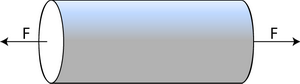
In plane stress, one of the principal stresses is zero but there are three finite strains. An example of this is the surface of a thin walled, pressurised cylinder, where the principal stress normal to the surface has a value of zero. More generally, plane stress conditions occur in sheet metal forming when a thin sheet is subjected to uniaxial or biaxial tension.

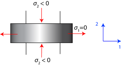
Plastic deformation in plane stress

Consider the uniaxial tensile behaviour of a sheet.

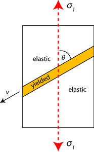
Plastic flow will result once a critical stress is reached. Due to the constraint of neighbouring elastic material, the plastically deforming material forms in a band across the sheet at a characteristic angle to the axis of loading.

\[{\sigma _1} \ne 0{\rm{ , }}{\sigma _{\rm{2}}} = {\sigma _3} = 0\]

At the boundary between the elastic and the yielded material, longitudinal strains must match for continuity. Therefore, they must be zero since strain is effectively zero in the elastic regions.

Plastic strain along v is zero: δε_vv= 0

From the Levy-Mises equations \[{{\delta {\varepsilon _1}} \over {{\sigma _1}}} = {{\delta {\varepsilon _2}} \over { - {\raise0.5ex\hbox{$\scriptstyle 1$} \kern-0.1em/\kern-0.15em \lower0.25ex\hbox{$\scriptstyle 2$}}{\sigma _1}}} = {{\delta {\varepsilon _3}} \over { - {\raise0.5ex\hbox{$\scriptstyle 1$} \kern-0.1em/\kern-0.15em \lower0.25ex\hbox{$\scriptstyle 2$}}{\sigma _1}}}\], and so \(\delta {\varepsilon _1} = - 2\delta {\varepsilon _2}\) in the plane of the sheet.

Hence if we let δε₁= +2 units of plastic strain, δε₂= –1 unit of plastic strain.

Therefore, on a Mohr's circle, we have:

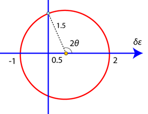
and the longitudinal strain δε is zero, i.e. δε_vv= 0, at an angle θ with respect to the direction parallel to σ₁.

From the diagram,

\[\cos \left( {180 - 2\theta } \right) = {{0.5} \over {1.5}} = {1 \over 3}\]

\[ \Rightarrow {\rm{ }}\theta = {\raise0.5ex\hbox{$\scriptstyle 1$} \kern-0.1em/\kern-0.15em \lower0.25ex\hbox{$\scriptstyle 2$}}{\cos ^{ - 1}}\left( { - {\raise0.5ex\hbox{$\scriptstyle 1$} \kern-0.1em/\kern-0.15em \lower0.25ex\hbox{$\scriptstyle 3$}}} \right) = {54.74^ \circ }\]

and so the longitudinal strain increment is δε_vv = 0 at an angle of with respect to σ₁.
 

This phenomenon is well known in mild steel. The bands created are known as Lüders bands. These bands require less stress for their propagation than for their formation because of the freeing of dislocations from their solute atmospheres.

     

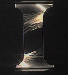
(Lüders bands formation in steel, contributed by Mike Meier, University of California, Davis.)

It is worth noting that Lüders bands occur in certain types of steel, such as low carbon steel (mild steel), but not in other metallic alloys, such as aluminium alloys or titanium alloys. This is because plastic strain localisation is normally suppressed by work hardening, which tends to make plastic flow occur rather uniformly in a metal, particularly in the early stages of plastic flow, i.e., just after yield has taken place.

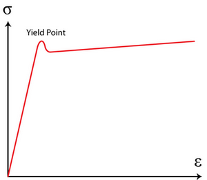
However, in certain types of low carbon steel at room temperature, Cottrell atmospheres of carbon atoms which have been able to segregate preferentially to dislocation cores pin dislocations until the upper yield point is reached. Once the upper yield point is reached, there is a load drop and then a sudden burst of plastic straining at a constant externally applied load, as cascades of dislocations are able escape their Cottrell atmospheres. This is clearly rather specialised behaviour, caused by the ability of carbon atoms to diffuse relatively easily interstitially in these steels, but it is actually necessary behaviour for the formation of Lüders bands.

Conventional work hardening in metallic alloys in the early stages of plastic deformation makes any strain localisation (as demonstrated by the formation of Lüders bands) unlikely. This is also the case for pure metals, and for metals at high temperature, where large plastic strains can occur without a significant load increase once plastic deformation begins.

Therefore, Lüders bands only form if a limited burst of plastic straining is able to take place at constant load. Mild steels heated to sufficiently high temperatures (> 400 °C) and then tensile tested do not exhibit Lüders bands.

 

• Plane strain

Much deformation of practical interest occurs under a condition that is nearly, if not exactly, one of plane strain, i.e. where one principal strain (say ε₃) is zero so that δε₃=0.

Plane strain is applicable to rolling, drawing and forging where flow in a particular direction is constrained by the geometry of the machinery, e.g. a well-lubricated die wall.

A specific example of this is in rolling, where the major deformation occurs perpendicular to the roll axis. The material becomes thinner and longer but not wider. Frictional stresses parallel to the rolls (i.e. in the width direction) prevent deformation in this direction and hence a plane strain condition is produced where δε₃=0. This can be seen in the animation below.

HOT ROLLING

Reproduced from Materials Selection and Processing CD, by A.M.Lovatt, H.R.Shercliff and P.J.Withers.

 

Plastic deformation in plane strain

Here, one principal strain is zero. Let this be ε₃. Then δε₃= 0.

From the Levy-Mises equation, \[{{\delta {\varepsilon _1}} \over {{\sigma _1} - {1 \over 2}\left( {{\sigma _2} + {\sigma _3}} \right)}} = {{\delta {\varepsilon _2}} \over {{\sigma _2} - {1 \over 2}\left( {{\sigma _3} + {\sigma _1}} \right)}} = {{\delta {\varepsilon _3}} \over {{\sigma _3} - {1 \over 2}\left( {{\sigma _1} + {\sigma _2}} \right)}} \ne 0\] it follows that \({\sigma _3} = {\textstyle{1 \over 2}}\left( {{\sigma _1} + {\sigma _2}} \right)\) in order to avoid \({{\delta {\varepsilon _1}} \over {{\sigma _1} - {1 \over 2}\left( {{\sigma _2} + {\sigma _3}} \right)}}\) = 0

Hence σ₃ is the mean of σ₁ and σ₂. By convention we define σ₁ > σ₂ σ₁ > σ₃ > σ₂. Therefore the maximum shear stress in the σ₁- σ₂ plane is at 45° to the axes and has magnitude \({{{\sigma _1} - {\sigma _2}} \over 2}\) .

If we now examine the Tresca and von Mises yield criteria, we find:

• Tresca \({{{\sigma _1} - {\sigma _2}} \over 2}\) = k = \({Y \over 2}\)    (k = shear yield stress and Y = uniaxial yield stress)
• von Mises \({\left( {{\sigma _1} - {\sigma _2}} \right)^2} + {\left( {{\sigma _2} - {\sigma _3}} \right)^2} + {\left( {{\sigma _3} - {\sigma _1}} \right)^2} = 6{k^2} = 2{Y^2}\)

$${\rm{If}\;\;\sigma _3} = {\textstyle{1 \over 2}}\left( {{\sigma _1} + {\sigma _2}} \right),{\rm{ }}{\textstyle{3 \over 2}}{\left( {\sigma {}_1 - {\sigma _2}} \right)^2} = 6{k^2} = 2{Y^2}$$

$$ \Rightarrow \left( {{\sigma _1} - {\sigma _2}} \right) = 2k = {{2Y} \over {\sqrt 3 }}$$

Therefore, if we have plane strain, the Tresca yield criterion and the von Mises yield criterion have the same result expressed in terms of k. It is unnecessary to specify which criterion we are using, provided we use k.

 

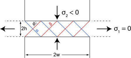
Consider a metal in uniaxial compression where plastic strain only takes place in the 1-2 plane. There is no friction between the work piece and the die faces. (To achieve this experimentally, a sample should be wide in the 3 direction).

-->

\[ \Rightarrow {\rm{ }}{\sigma _{{\rm{ij}}}} = {\rm{ }}\left( {\matrix{ {{\sigma _1}} & 0 & 0 \cr 0 & {{\sigma _2}} & 0 \cr 0 & 0 & {{{{\sigma _1} + {\sigma _2}} \over 2}} \cr } } \right)\]

 

Hydrostatic stress:

\[{\sigma _H} = - p = {{{\sigma _1} + {\sigma _2}} \over 2} = {\sigma _3}\]

where p is the hydrostatic pressure.

So at yield, we have \({{{\sigma _1} - {\sigma _2}} \over 2}\) = \(k\) and since \({{{\sigma _1} + {\sigma _2}} \over 2}\) = \(- p\), we have

\[{\sigma _1} = - p + k = 0\]

\[{\sigma _2} = - p - k = - 2k\]    since p=k at yield

\[{\sigma _3} = - p\]

 

So for this example, the stress tensor is

\[{\rm{ }}{\sigma _{{\rm{ij}}}} = {\rm{ }}\left( {\matrix{ { - p} & 0 & 0 \cr 0 & { - p} & 0 \cr 0 & 0 & { - p} \cr } } \right) + \left( {\matrix{ k & 0 & 0 \cr 0 & { - k} & 0 \cr 0 & 0 & 0 \cr } } \right)\]

which is the sum of hydrostatic stress (which can vary in magnitude through the object) and deviatoric pure shear stress (which has the same value throughout the material).

The directions of maximum shear therefore lie at 45° to σ₁ and σ₂. These are slip lines along which plastic flow occurs.

We are avoiding additional complexities such as work hardening by assuming the materials are rigid-plastic.

Slip Line Field Theory

This approach is used to model plastic deformation in plane strain only for a solid that can be represented as a rigid-plastic body. Elasticity is not included and the loading has to be quasi-static. In terms of applications, the approach now has been largely superseded by finite element modelling, as this is not constrained in the same way and for which there are now many commercial packages designed for complex loading (including static and dynamic forces plus temperature variations). Nonetheless, slip line field theory can provide analytical solutions to a number of metal forming processes, and utilises plots showing the directions of maximum shear stress in a rigid-plastic body which is deforming plastically in plane strain. These plots show anticipated patterns of plastic deformation from which the resulting stress and strain fields can be estimated.

The earlier analysis of plane strain plasticity in a simple case of uniaxial compression established the basis of slip line field theory, which enables the directions of plastic flow to be mapped out in plane strain plasticity problems.

There will always be two perpendicular directions of maximum shear stress in a plane. These generate two orthogonal families of slip lines called α-lines and β-lines. (Labelling convention for α and β lines.)

 

 

Experimentally, these lines can be seen in a realistic plastic deformation situation, e.g.

• Polyvinyl chloride (PVC) viewed between crossed polars
  
• Nitrogen-containing steels can be etched using Fry’s reagent to reveal regions of plastic flow in samples such as notched bars and thick walled cylinders.
  
• Under dull red heat in forging, we see a distinct red cross caused by dissipation of mechanical energy on slip planes.

To develop slip line field theory to more general plane strain conditions, we need to recognise that the stress can vary from point to point.

Therefore, p can vary, but k is a material constant. As a result of this, directions of maximum shear stress and the directions of principal stresses can vary along a slip line.

 

Hencky relations

These equations arise from consideration of the equilibrium equations in plane strain.

p + 2kφ = constant along an α line

p – 2kφ = constant along a β line

 Click here for the derivation.

We can apply these relations to the classic problem of indentation of a material by a flat punch. This is important in hardness testing, in foundations of buildings and in forging.

In more general cases, slip lines do not intersect external boundaries at 45° because of friction. In the extreme case, sticking friction occurs (a perfectly rough surface) and slip lines are at 90° to the surface.

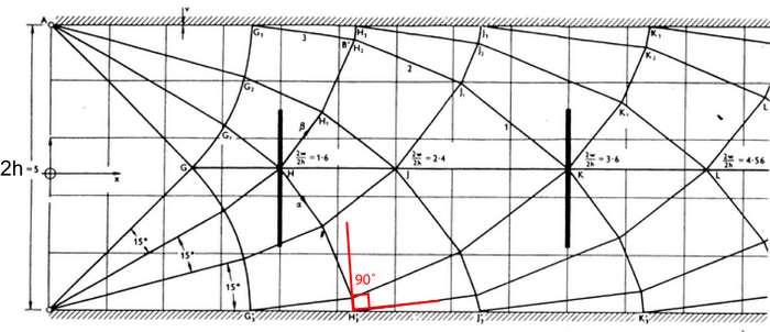
Slip-line field for compression between a pair of rough parallel platens [1]

The slip line patterns above are very useful for analysing plane strain deformation in a rigid-plastic isotropic solid. Arrival at this slip-line pattern is rather complex. They are either derived from model experiments in which the slip-line field is apparent or they are postulated from experience of problems with similar geometry.

For a slip line to be a valid solution (but not necessarily a unique solution) the stress distribution throughout the whole body, not just in the plastic region, must not violate stress equilibrium nor must it violate the yield criterion outside the slip-line field.

The resultant velocity field must also be evaluated to ensure that strain compatibility is satisfied and matter is conserved.

These are stringent conditions and mean that obtaining a slip-line field solution is often not simple.

Instead, it is useful to take a more simple approach to analysing deformation processing operations where one or another of the stringent conditions are relaxed to give useful approximate solutions for part of the analysis.

 

Work Formula Method

When deforming a body, work has to be done by the applied forces.  In the simplest case, the work done can be estimated from the magnitude of the applied stress(es) and the extent of the deformation. This is analogous to simple mechanics in which the work done is equal to force applied multiplied by the distance moved.  Clearly, this simple approach assumes, in the first instance, that all the work done by the applied forces results in deformation; this can be called “useful” work.  If it is assumed that all the work done is useful, then the work formula approach leads to an underestimate of the actual forces needed, i.e. a “lower bound”.  In other words, it would not be possible to deform the body if at least those forces were not applied and hence that work was not done.  In practice, frictional forces need to be overcome and heating of the body occurs due to the internal micro-mechanisms of deformation.  This non-useful work is called “redundant” work and estimates can be made to allow for this, and so better approximations for the necessary forces can be made.

Consider a uniaxial tensile deformation process:

In this process, σ₁ = Y, σ₂ = σ₃ = 0 and Y = uniaxial yield stress.

 

-->

 

Suppose that at some instant, the bar is of length l and of cross-sectional area A
V = Al

If the bar extends by an amount δl, the increment of work done/unit volume, δw, is

$${{F\delta l} \over V} = {{YA\delta l} \over {Al}} = \delta w$$

\[\delta w = {{Y\delta l} \over l}\]

So if the bar extends from length l₀ to l₁, total work done/unit volume is

\[\int {\delta w} = Y\int_{{l_0}}^{{l_1}} {{{{\rm{d}}l} \over l}} = Y\ln {{{l_1}} \over {{l_0}}}\]

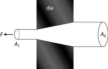
This can be applied to wire drawing.

In wire drawing, a tensile force is applied to the product rather than a compressive force applied to the billet (such as in extrusion for example).

 

-->

 

To extend the wire by distance l₁, we have to feed in a length l₀ to the die where A₁l₁ = A₀l₀ by conservation of volume.

Work done by F = Fl₁

Volume of metal = A₁l₁drawn by l₁

Work done \( = Y{A_1}{l_1}\ln \) \({{{l_1}} \over {{l_0}}}\) = \(F{l_1}\)

\[ \Rightarrow {F \over {{A_1}}} = \sigma = Y\ln {{{l_1}} \over {{l_0}}} = Y\ln {{{A_0}} \over {{A_1}}}\]

where σ = stress required, the drawing stress.

 

Therefore we can estimate the maximum reduction possible with perfect lubrication.

If there is no work hardening, \(\sigma \le Y\) then the maximum reduction occurs when
σ = Y \( \Rightarrow \ln \) \({{{A_1}} \over {{A_0}}}\) = 1   

\[ \Rightarrow {{{A_0}} \over {{A_1}}} = 2.72\]   (e to 3 s.f.)

\[ \Rightarrow {{{A_1}} \over {{A_0}}} = 0.37\]

63% is therefore the maximum possible reduction of cross-sectional area with a perfect wire-drawing operation for a rigid-plastic material. Work hardening causes this to increase to a slightly higher value. Friction between the wire and the die reduces this value, causing redundant work – work in excess of the minimum necessary to cause the deformation.

 

In practice, the best reduction obtainable with real dies and good lubrication is approximately 50%.

To allow for redundant work, we can apply empirical corrections, e.g. by using a value of efficiency, η:

\[\eta = {{{\rm{Work\; formula\; estimate}}} \over {{\rm{Actual\; total\; work}}}}\]

Typical values of η are:

• extrusion         η = 45 – 55%
  
• wire drawing   η = 50 – 65%
  
• rolling               η = 60 – 80%

Clearly, the work formula method gives a lower band to the true force required for a given deformation processing operation because we are neglecting ‘redundant work.’

For metalworking, it is often preferable to have an overestimate of the load required in order to be sure that a given operation or process is possible.

 

Limit Analysis

The concept of a lower bound has been introduced with reference to the work formula approach to analyse deformation. This approach generally results in an underestimate of the required load. Clearly, there also will be an “upper bound”, i.e. an overestimate of the load that needs to be applied to effect a given deformation. The two approaches together are called “limit analysis” since the actual loads required will lie between the lower and upper bounds. In practice, limit analysis is much easier to apply to a problem than the slip-line field approach and can be reasonably accurate. The upper bound is particularly useful for the study of metalworking processes in which it is essential to ensure sufficient forces are applied to cause the required deformation. In contrast, the lower bound is valuable in engineering where failure of a component must be avoided and hence an estimate of the minimum collapse load is needed.

The approach taken for estimating the upper bound is based on suggesting a likely deformation pattern, i.e. lines along which slip would be expected to occur for a given loading situation. Then the rate at which energy is dissipated by shear along these lines can be calculated and equated to the work done by an (unknown) external force. By refining the geometry of the deformation pattern, the minimum upper bound can be determined. Frictional forces can be accommodated in this approach. The approach utilises hodographs, which are self-consistent plots of velocity for different regions within a body being deformed; the different regions are assigned by considering how the overall body will deform for a particular deformation process and their relative velocities are estimated by assuming that the applied external force has unit velocity.

For both upper- and lower-bounds, one of the following two conditions has to be satisfied:

• geometrical compatibility between internal and external displacements or strains. This is usually concerned with kinetic conditions – velocities must be compatible to ensure no gain or loss of material at any point.
  
  
• stress equilibrium i.e. the internal stress fields must balance the externally applied stresses (forces).

The basis of limit analysis rests upon two theorems, which can be proved mathematically. In simple terms, these theorems are:

1. Lower Bound: any stress system in which the applied forces are just sufficient to cause yielding.
   
   
2. Upper Bound: Any velocity field that can operate is associated with an upper bound solution.
   

 Example 1: Notched bar in tension.

 Example 2: Notched bar in plane bending.

 

• Notched bar in tension

The plane strain condition is satisfied when breath, b » h, the depth of the bar.

Lower-Bound:

Find a stress system, e.g. σ = 0 in the length of the bar where there is the notch, σ = 2k elsewhere.

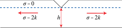
Therefore, for a breadth b, P = 2khb = load = stress × area

Upper-Bound:

Postulate a suitable simple deformation pattern.

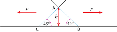
Assume yielding by slip on 45º shear planes with shear yield stress k. Let displacement along shear plane AB = δx.

Then internal work done = \( {k.\left| {AB} \right|b\delta x} = k\sqrt 2 bh\delta x\), where the force is \( k\left| {AB} \right|b \) acting on the shear plane AB.

Distance moved by the external load \(P = \delta x\cos {45^ \circ }\) = \(\frac{{\delta x}}{{\sqrt 2 }}\)

\( \Rightarrow P \) \(\frac{{\delta x}}{{\sqrt 2 }}\) = \(k\sqrt 2 bh\delta x\)

\( \Rightarrow P = 2kbh\)

So, here we obtain the same result for the upper bound and lower bound \( \Rightarrow P = 2kbh\) is the true failure load, the load required to cause plastic flow.

 

• Notched bar in plane bending

Lower-Bound:

The area immediately under the notch, above the neutral axis is in tension σ = 2k. The area below the neutral axis is in compression σ = 2k.

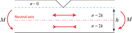
where:

           h = thickness of slab beneath the notch.

           \(2k.\) \(\frac{h}{2}\)\(.b\) = magnitude of forces in tensile and compressive regions.
           \(\frac{h}{2}\) = distance between the two.

Equating the couples, \(M = \) \(\left( {2k.\frac{h}{2}.b} \right)\) \(\frac{h}{2}\) = \(0.5k{h^2}b\)

Upper-Bound:

Assume failure occurs by sliding around a ‘plastic hinge’ along a circular arc of length l and radius r.

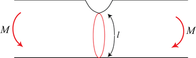
If the rotation is δθ, the internal work done \( = k.lb.r\delta \theta \) along one arc.

External work = Mδθ by one moment.

\[ \Rightarrow M = klbr\]

where no assumptions have been made regarding l and r.

The upper bound theorem states that whatever values are taken for l and r will lead to an upper bound. Clearly we wish to find the lowest possible value.

 

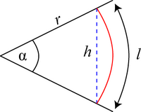
From the above geometry,

\(l = r\alpha \)    and     \(r = \) \(\frac{h}{{2\sin {\raise0.7ex\hbox{$\alpha $} \!\mathord{\left/ {\vphantom {\alpha 2}}\right.\kern 2pt} \!\lower0.7ex\hbox{$2$}}}}\)

\[ \Rightarrow M = \frac{{k{h^2}b}}{4}\frac{\alpha }{{{{\sin }^2}{\raise0.7ex\hbox{$\alpha $} \!\mathord{\left/ {\vphantom {\alpha 2}}\right.\kern 1pt} \!\lower0.7ex\hbox{$2$}}}}\]

and so to find the lowest possible value of M, we minimise the function \(\frac{\alpha }{{{{\sin }^2}{\raise0.7ex\hbox{$\alpha $} \!\mathord{\left/ {\vphantom {\alpha 2}}\right.\kern 1pt} \!\lower0.7ex\hbox{$2$}}}}\)

Let  \(Y = \) \(\frac{\alpha }{{{{\sin }^2}{\raise0.7ex\hbox{$\alpha $} \!\mathord{\left/ {\vphantom {\alpha 2}}\right.\kern 1pt} \!\lower0.7ex\hbox{$2$}}}}\)

\(\frac{{{\rm{d}}Y}}{{{\rm{d}}\alpha }} = \frac{1}{{{{\sin }^4}{\alpha \mathord{\left/ {\vphantom {\alpha 2}} \right. \kern 1pt} 2}}}\left\{ {{{\sin }^2}\frac{\alpha }{2} - 2\frac{\alpha }{2}\cos \frac{\alpha }{2}\sin \frac{\alpha }{2}} \right\}\)

       = 0      when    \(\sin \frac{\alpha }{2} = \alpha \cos \frac{\alpha }{2}\)

\[ \Rightarrow \tan \frac{\alpha }{2} = \alpha \]

\[ \Rightarrow M = \frac{{k{h^2}b}}{4}.\frac{1}{{\sin {\raise0.5ex\hbox{$\scriptstyle \alpha $} \kern-0.1em/\kern-0.15em \lower0.25ex\hbox{$\scriptstyle 2$}}\cos {\raise0.5ex\hbox{$\scriptstyle \alpha $} \kern-0.1em/\kern-0.15em \lower0.25ex\hbox{$\scriptstyle 2$}}}} = {\raise0.7ex\hbox{$1$} \!\mathord{\left/ {\vphantom {1 2}}\right.\kern 1pt} \!\lower0.7ex\hbox{$2$}}\frac{{k{h^2}b}}{{\sin \alpha }} \cong 0.69k{h^2}b\]

Taking the lower bound and the upper bound as limits, we therefore find

\[ \Rightarrow 0.5 \le \frac{M}{{k{h^2}b}} \le 0.69\]

This forms a good example of constraining the value of the external force between lower bound and upper bound. It is also a good example of how to produce a lower limit on an upper bound calculation.

 

• Hodographs I

A hodograph is a diagram showing the relative velocities of the various parts of a deformation process.

To analyse a complicated deformation process with many shear planes, it is worth looking at the basic equation for the rate of energy dissipation in an upper bound situation in more detail.

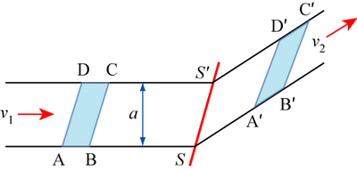
ABCD is distorted into A'B'C'D' by shear along \(\overrightarrow {SS`} \) at a velocity \(\underline {{v_s}} \) in the metal.

Suppose ABCD moves towards the shear plane SS' at a velocity \({v_1}\) and suppose that there is a pressure P acting on the area al (where l is the dimension out of the plane of the paper) helping to cause this movement.

Rate of performance of work externally \( = pal\left| {\underline {{v_1}} } \right|\)

Rate of performance of work internally \( = k\left| {SS`} \right|l\left| {\underline {{v_s}} } \right|\)

since the only internal work assumed to occur is that required to effect the shear deformation so that ABCD → A'B'C'D'.

Equating these, \( \Rightarrow pa\left| {\underline {{v_1}} } \right| = k\left| {SS`} \right|\left| {\underline {{v_s}} } \right|\)

\( \Rightarrow pa = k\left| {SS`} \right|\frac{{\left| {\underline {{v_s}} } \right|}}{{\left| {\underline {{v_1}} } \right|}}\)

Simple vector algebra relates v₁, v₂ and v_s as on the diagram below:

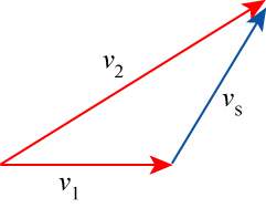
If in a deformation process there are n such shear planes of the type SS',

then \(pa = k\sum\limits_n {\left| {SS_n^`} \right|\left| {{v_{sn}}} \right|} \) setting \(\left| {\underline {{v_1}} } \right| = 1.0\), i.e. unit velocity.

Rules for constructing a hodograph

The animation below illustrates the seven rules for constructing a hodograph, for the case of a constrained punch.

An analysis of the geometry of the hodograph enables an upper bound for the applied force to be calculated.

Let Oq be a velocity vector of unit magnitude in the hodograph, i.e. ν_Oq = 1
Due to the dead metal zone, Q and Q' move at the same velocity.
O is a stationary component of the system, anywhere in the surrounding perfectly rigid metal which has not yielded at all.
Oq and Oq' are in essence vectors defining the motion of particles in region Q'.
Or is velocity of a particle in region R.
q'r is a vector defining the shear velocity parallel to Q'R.
Os is velocity of a particle in region S.
rs is a vector defining the shear velocity parallel to RS.

Hence,

\[{v_{Or}} = \frac{1}{{\tan \theta }}{\rm{ ,\; }}{v_{q'r}} = \frac{1}{{\sin \theta }}{\rm{\; and \; }}{v_{Os}} = {v_{rs}} = \frac{1}{{2\sin \theta }}\]

Using the rate of performance of work formula we have:

\[p\left( {\frac{b}{2}} \right) = k\left\{ {Q'R{v_{q'r}} + OR{v_{Or}} + RS{v_{rs}} + OS{v_{Os}}} \right\}\]

where Q'R is the length of the line dividing regions Q' and R, OR is the length of the line dividing regions O and R, RS is the length of the line dividing regions R and S and OS is the length of the line dividing regions O and S

\[p\left( {\frac{b}{2}} \right) = kb\left\{ {\frac{1}{{2\cos \theta }}.\frac{1}{{\sin \theta }} + 1.\frac{1}{{\tan \theta }} + \frac{1}{{2\cos \theta }}.\frac{1}{{2\sin \theta }} + \frac{1}{{2\cos \theta }}.\frac{1}{{2\sin \theta }}} \right\}\]

\[ = kb\left\{ {\frac{1}{{\sin \theta \cos \theta }} + \frac{{\cos \theta }}{{\sin \theta }}} \right\} = kb\left\{ {\frac{{1 + {{\cos }^2}\theta }}{{\cos \theta \sin \theta }}} \right\}\]

\[ \Rightarrow \frac{p}{{2k}} = \frac{{1 + {{\cos }^2}\theta }}{{\sin \theta \cos \theta }} = f\left( \theta \right)\]

\(\frac{{df}}{{d\theta }}\) = 0 and f is then a minimum when

\[\cos 2\theta = - \frac{1}{3}{\rm{ }} \Rightarrow {\rm{ }}\theta = {54.74^ \circ }{\rm{ when }}\sin \theta = \frac{{\sqrt 2 }}{{\sqrt 3 }}{\rm{ and }}\cos \theta = \frac{1}{{\sqrt 3 }}\]

minimum \(\frac{p}{{2k}}\)\( = 2\sqrt 2 = 2.83\) from this upper bound analysis.

 

When indenting using a sliding (frictionless) punch, we can postulate a different deformation pattern without the dead metal zone. The system also has a plane of symmetry and a hodograph can be constructed as follows:

As before, Oq = 1.0

Material in R travels in direction shown with velocity \(Or = \) \(\frac{1}{{\sin \theta }}\)

\(\left| {Or} \right| = \left| {rs} \right| = \) \(\frac{1}{{\sin \theta }}\)\( = \left| {st} \right| = \left| {Ot} \right|\)

\(\left| {Os} \right| = \) \(\frac{{2\cos \theta }}{{\sin \theta }}\)

\(\left| {qr} \right| = \) \(\frac{1}{{\tan \theta }}\) = \(\frac{{\cos \theta }}{{\sin \theta }}\)

Lengths in drawing of indent: \(QR = SO =\) \(\frac{b}{2}\)

\(OR = RS = ST = OT = \) \(\frac{b}{{4\cos \theta }}\)

We therefore have:

\(\frac{{pb}}{2}\) = \(k\left\{ {OR{v_{Or}} + RS{v_{rs}} + OS{v_{Os}} + ST{v_{st}} + TO{v_{tO}}} \right\}\)

\( = kb\) \(\left\{ {\frac{1}{{4\cos \theta }}.\frac{1}{{\sin \theta }} + \frac{1}{{4\cos \theta }}.\frac{1}{{\sin \theta }} + \frac{1}{2}.\frac{{2\cos \theta }}{{\sin \theta }} + \frac{1}{{4\cos \theta }}.\frac{1}{{\sin \theta }} + \frac{1}{{4\cos \theta }}.\frac{1}{{\sin \theta }}} \right\}\)

\( = kb \) \(\left\{ {\frac{1}{{\sin \theta \cos \theta }} + \frac{{\cos \theta }}{{\sin \theta }}} \right\}\)

\( \Rightarrow \) \(\frac{P}{{2k}}\) = \(\left\{ {\frac{{1 + {{\cos }^2}\theta }}{{\sin \theta \cos \theta }}} \right\}\) as before for the case of the constrained punch.

This analysis has assumed that no friction occurs at the punch face to cause particles in R to move parallel to OR. If there is friction, we can take it to be sticking friction, so that there is a shear stress k acting and slippage velocity \( = {v_{qr}}\)

\( \Rightarrow \) in this case \(\frac{P}{{2k}}\) = \(\left\{ {\frac{{2 + 3{{\cos }^2}\theta }}{{2\sin \theta \cos \theta }}} \right\}\)

\( \Rightarrow \) of the three possible upper bound solutions, the 'best' answer is \(\frac{P}{{2k}}\) = \(2\sqrt 2 = 2.83\)

This is a 10% overestimate of the true value of \(\frac{P}{{2k}}\) found from slip-line field theory.

• Hodographs II

Extrusion is an important working process. A simple form of extrusion used for non-ferrous metals involves a smooth square die.

We define extrusion ratio, R = ratio of areas.

\(R = \) \(\frac{{{A_0}}}{{{A_1}}}\) = \(\frac{H}{h}\) for plane strain (R > 1), e.g. R = 4 = 75% reduction in area.

For a square die with sliding on the die face in plane strain, the hodograph can be constructed as follows:

Click here for a full mathematical analysis of this hodograph.

An alternative approach to an extrusion hodograph assumes there is a 'dead metal' zone.

Then \(p\frac{H}{2}\) = \(k\left\{ {PQ{v_{PQ}} + DQ{v_{dq}} + QR{v_{qr}}} \right\}\)

After similar algebra to the previous example, we obtain

\[\frac{p}{{2k}} = \frac{1}{{2\left( {\sin \varphi - \cos \varphi } \right)}}\left\{ {\frac{{R + 1}}{{\sin \varphi }} - 2\left( {R - 1)\cos \varphi } \right)} \right\}\]

Minimising RHS, \(\cot \varphi = 1 - \) \(\frac{2}{{\sqrt {R + 1} }}\)

After more algebra, it is found that

\[\frac{{{p_{\min }}}}{{2k}} = 2\left( {\sqrt {R + 1} - 1} \right)\]

Note that for low R (< 4) this value is less than that for sliding on the die face, even if the die face is frictionless.

\( \Rightarrow \) For R < 4 this is a better upper bound solution for extrusion problems.

 Click here for a full mathematical analysis of this hodograph.

Finite Element Method

Finite element analysis (FEA) is an increasingly powerful computational technique in which the geometry of even a very complex body is represented by a mesh comprising a large number of discrete regions called finite elements. The elements are linked to each other at discrete points called nodes and different geometry elements (with varying numbers of nodes) can be selected for different types of problems. The use of FEA extends well beyond simple deformation since the approach can handle static and dynamic loading (with time-dependent changes in loads), two or three dimensional objects and different types of loading, e.g. thermal, electromagnetic as well as mechanical forces. Many commercial packages are now available.

The animation below depicts a finite-element simulation for the production of gudgeon pins. These are pins which hold a piston rod and a connecting rod together. The process consists of 4 stages [2]:

1. Upsetting
   
2. Indentation
   
3. Backward Extrusion
   
4. Punching – The base of the cup is punched out producing the gudgeon pin.

The simulation accounts for steps 1 to 3.

Summary

This module has presented different approaches to model plastic flow in metal forming operations, showing their relative importance and limitations. 

The approaches covered are:-

• Slip line field theory
  
• Work formula analysis
  
• Limit analysis and hodographs
  
• Finite element analysis

The backgrounds to the approaches have been summarised, and then examples presented to show how each can be used in practice to provide estimates of the necessary deformation loads for the various metal forming operations.

Questions

Deeper questions

The following questions require some thought and reaching the answer may require you to think beyond the contents of this TLP.

1. A specimen of sheet steel is tested in unequal biaxial tension, and Lüders bands form at 60° to one of the tensile axes. Show that the ratio between the two principal stresses in the plane of the sheet is 1:5.

   If the greater of these two principal stresses is 500 MPa and the steel obeys von Mises' yield criterion, show that the yield stress in uniaxial tension is 458 MPa.

2. Use a work formula approach to estimate the minimum pressure required to extrude aluminium curtain rail of I-section, 12 mm high with 6 mm wide flanges, all 1.6 mm thick, from 25 mm diameter bar stock.

   [The mean uniaxial yield stress for aluminium for heavy deformation at room temperature is 150 MPa. The minimum pressure, , required is given by the formula

   

   where  is the original cross-sectional area and  is the cross-sectional area of the extruded I-section].

3. The diagram below shows a possible deformation pattern for the direct plane-strain extrusion of a metal slab, initially 40 mm thick, through a symmetrical 45° tapering die, with an extrusion ratio of 2.The diagram shows half the deformation pattern and the angles BCD and CBD are both 45°. The distance AB is 15 mm. The width of the slab is 100 mm and its yield stress in pure shear is 150 MPa.

   

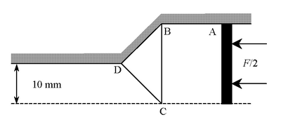
   Calculate an upper bound to the extrusion force F acting on the slab if the extrusion process is frictionless.

Going further

Books:

[1] W. Johnson and P.B. Mellor, Engineering Plasticity, Van Nostrand Reinhold Comapny Ltd., 1978.

[2] G.W. Rowe, C.E. Sturgess, P. Hartley and I. Pillinger, Finite-Element Plasticity and Metalforming Analysis, Cambridge University Press, 1991.

 

---

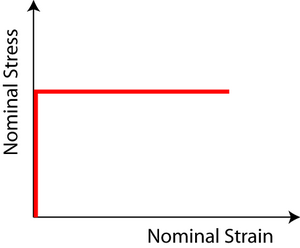
Rigid-plastic

A rigid-plastic material is defined as a material exhibiting no elastic deformation and perfect plastic deformation. Compared to a real metal, all elastic behaviour and strain hardening effects are ignored.

 

Hencky relations

The equilibrium equations for plane strain are:

$$\frac{{\partial {\sigma _{xx}}}}{{\partial x}} + \frac{{\partial {\tau _{xy}}}}{{\partial y}} = 0$$

$$\frac{{\partial {\tau _{xy}}}}{{\partial x}} + \frac{{\partial {\sigma _{yy}}}}{{\partial y}} = 0$$

Unless τ_xy = ± k, where k is the shear yield stress, the x- and y-directions (or axes) will not correspond to the directions of the α- and β-slip lines, which are themselves at ± 45° to the directions of principal stresses acting on the element.

In general, we need to examine the stresses on a small curvilinear element in the x-y plane upon which a shear stress and a hydrostatic stress are acting, and where the principal stresses are – p – k and – p + k for a situation where there is plane strain compression, such as in forging or indentation in which k is a constant but p can vary from point to point:

We can then identify on this diagram the directions of principal stress σ₁ and σ₂ (remembering that σ₁ > σ₂), and which of the lines are α-lines and which are β-lines. We can also specify the angle φ of the α-lines with respect to the x-axis:

Suppose that the α-slip line passing through the element makes an angle φ with respect to reference x- and y-axes, as in the above diagram. The β-slip line must then make an angle of 90° + φ with respect to the x-axis, so that an anticlockwise rotation from the α-slip line to the β-slip line crosses the direction of maximum principal stress, σ₁.

The direction parallel to the principal stress σ₁ makes an angle of 45° + φ with respect to the x-axis and the direction parallel to the principal stress σ₂ makes an angle of 135° + φ º 45° – φ with respect to the x-axis.

On a Mohr’s circle, this all looks like:

where A and B represent the stress states along the α- and β-lines respectively.

Hence, from the above,

$$\begin{array}{l} {\sigma _{xx}} = - p - k\sin 2\varphi \\ {\sigma _{yy}} = - p + k\sin 2\varphi \\ {\tau _{xy}} = k\cos 2\varphi \end{array}$$

while the tensile stress in the z-direction in plain strain plastic yielding is simply:

$$\frac{1}{2}\left( {{\sigma _{xx}} + {\sigma _{yy}}} \right) = - p$$

Substituting these expressions into the equilibrium equations

$$\frac{{\partial {\sigma _{xx}}}}{{\partial x}} + \frac{{\partial {\tau _{xy}}}}{{\partial y}} = 0$$

$$\frac{{\partial {\tau _{xy}}}}{{\partial x}} + \frac{{\partial {\sigma _{yy}}}}{{\partial y}} = 0$$

and recognising that k is a constant independent of x and y, we obtain two equations for p and φ as a function of x and y:

$$\begin{array}{l} - \frac{{\partial p}}{{\partial x}} - 2k\cos 2\varphi \frac{{\partial \varphi }}{{\partial x}} - 2k\sin 2\varphi \frac{{\partial \varphi }}{{\partial y}} = 0\\ - 2k\sin 2\varphi \frac{{\partial \varphi }}{{\partial x}} - \frac{{\partial p}}{{\partial y}} + 2k\cos 2\varphi \frac{{\partial \varphi }}{{\partial y}} = 0 \end{array}$$

For φ = 0°, in which case the α and  β lines coincide with the external x- and y-axes respectively at a particular position, these equations become

$$(1)\;\;{\rm{ }}\frac{\partial }{{\partial x}}\left( {p + 2k\varphi } \right) = 0$$ $$(2)\;\;{\rm{ }}\frac{\partial }{{\partial y}}\left( {p - 2k\varphi } \right) = 0$$

Integrating these equations we find

$$\begin{array}{l} (1)\;\;{\rm{ }}p + 2k\varphi = {f_1}(y) + {C_1}\\ (2)\;\;{\rm{ }}p - 2k\varphi = {f_2}(x) + {C_2} \end{array}$$

as the most general form of the solutions of these two partial differential equations. However, we know that when φ is exactly zero, p must have the same value in both (1) and (2). Hence it follows that f₁(x) = f₂(y) = 0.

In general for points in a slip-line field we have therefore proved that the Hencky relations have to be satisfied:

Hencky relations The hydrostatic pressure p varies linearly with the angle φ turned by a slip line. p + 2kφ is constant along an α line p – 2kφ is constant along a β line where the angle φ is in radians.

 

Extrusion: assuming sliding on die face

The mathematics behind the equation for p_min:

 

To analyse this situation, it is convenient to define angle Osr in the hodograph as θ and angle Oqr as φ . Thus the plane of shear between R and S makes an angle θ with the horizontal extrusion axis and the plane of shear between Q and R makes an angle φ with the horizontal extrusion axis.

Let Oq be a velocity vector of unit magnitude in the hodograph, i.e. ν_Oq = 1

Hence,

\[{\nu _{Or}} = \tan \phi ,\;\;{\nu _{qr}} = \frac{1}{{\cos \phi }},\;\;{\nu _{rs}} = \frac{{\tan \phi }}{{\sin \theta }}\;\;and\;\; {\nu _{Os}} = R\]

where R is the extrusion ratio = H/h

From the diagram of the extrusion process it follows that

\[\frac{h}{{2\tan \theta }} = \frac{H}{{2\tan \phi }}{\rm{ \;\; and\;\; so \;\; }}R = \frac{H}{h} = \frac{{\tan \phi }}{{\tan \theta }}\]

 

Applying the general formula

$$pa = k\sum\limits_n {\left| {{\rm{SS}}{'_n}} \right|} \left| {{v_{sn}}} \right|$$

we then have

\[p\frac{H}{2} = k\left\{ {{\rm{QR}}{v_{qr}} + {\rm{RS}}{v_{rs}}} \right\}\]

where QR is the length of the line dividing regions Q and R and RS is the length of line dividing regions R and S in the diagram of the extrusion operation.

 

Now,

$${\rm{QR}} = \frac{H}{{2\sin \varphi }}{\rm{ \;\; and \;\; RS}} = \frac{H}{{2\sin \theta }}$$

and so

$$R = \frac{{{A_0}}}{{{A_1}}} = \frac{H}{h}$$

$$p\frac{H}{2} = k\left\{ {\frac{H}{{{\rm{2sin}}\phi }}.\frac{1}{{\cos \phi }} + \frac{h}{{{\rm{2sin}}\theta }}.\frac{{\tan \phi }}{{\sin \theta }}} \right\}$$

$$ = k\left\{ {\frac{H}{{{\rm{2sin}}\phi }}.\frac{1}{{\cos \phi }} + \frac{H}{{{\rm{2sin}}\theta }}.\frac{{\tan \theta }}{{\sin \theta }}} \right\}$$

substituting for h tanφ. Hence,

$$p = k\left\{ {\frac{1}{{{\rm{sin}}\varphi \cos \varphi }} + \frac{1}{{\sin \theta \cos \theta }}} \right\}$$

Now,

$$\frac{1}{{{\rm{sin}}\varphi \cos \varphi }} = \frac{{{{\sin }^2}\varphi + {{\cos }^2}\varphi }}{{{\rm{sin}}\varphi \cos \varphi }} = \tan \varphi + \frac{1}{{\tan \varphi }} \equiv R\tan \theta + \frac{1}{{R\tan \theta }}$$

and likewise

$$\frac{1}{{{\rm{sin}}\theta \cos \theta }} = \tan \theta + \frac{1}{{\tan \theta }}$$

whence

$$p = k\left( {R + 1} \right)\left\{ {\tan \theta + \frac{1}{{R\tan \theta }}} \right\}$$

and so to obtain the lowest value of p, p_min, we can minimise this function with respect to tan θ. If we let tan θ = x, then

$$p = k\left( {R + 1} \right)\left\{ {x + \frac{1}{{Rx}}} \right\}$$

and so the function is a minimum when R x² = 1. Hence,

$$\frac{{{p_{\min }}}}{{2k}} = \frac{{\left( {R + 1} \right)}}{{\sqrt R }}$$

Thus, for this model of extrusion in which there is sliding on the die face, we find:

Extrusion Ratio, R ( = H/h)	1.33	2	4	10
Reduction, r	25%	50%	75%	90%
pmin/2k	2.02	2.12	2.50	3.48
0.8 + 1.5 ln R	0.29	0.69	1.39	2.30

The graph below shows the estimates of p/2k as a function of R, assuming sliding on die face. The empirical equation used in practice 0.8 + 1.5 ln R is plotted for comparison.

Extrusion: assuming dead metal zone at 45°

The mathematics behind the equation for p_min:

 

Mathematically, this is more complicated than the situation in which there is sliding on the die face.

In the hodograph, it is convenient to define angle Orq in the hodograph as θ and angle rpq as φ. By definition, angle pOq is 45°.

Applying the general formula

$$pa = k\sum\limits_n {\left| {{\rm{SS}}{'_n}} \right|} \left| {{v_{sn}}} \right|$$

we then have

\[p\frac{H}{2} = k\left\{ {{\rm{PQ}}{v_{pq}} + {\rm{DQ}}{v_{dq}} + {\rm{QR}}{v_{qr}}} \right\}\]

where PQ is the length of the line dividing regions P and Q, DQ is the length of line dividing regions D and Q and QR is the length of line dividing regions Q and R in the above diagram showing the extrusion operation.

Now,

$${\rm{PQ}} = \frac{H}{{2\sin \varphi }}{\rm{ , DQ}} = \frac{1}{{\sqrt 2 }}\left( {H - h} \right){\rm{ \;\; and\;\; QR}} = \frac{h}{{2\sin \theta }}$$

In the hodograph, Op = 1 and Or = R, the extrusion ratio, i.e., ν_Op = 1 and ν_Or = R.

From triangle Opq, we having, using the sine rule,

\[\frac{{pq}}{{\sin {{45}^ \circ }}} = \frac{1}{{\sin \left( {\phi - {{45}^ \circ }} \right)}},{\rm{ \;\; and \;\;so \;\; }}{v_{pq}} = \frac{1}{{\sin \phi - \cos \phi }}\]

Likewise,

\[\frac{{dq}}{{\sin \left( {{{180}^ \circ } - \phi } \right)}} = \frac{1}{{\sin \left( {\phi - {{45}^ \circ }} \right)}},{\rm{ \;\; and \;\;so \;\; }}{v_{dq}} = \frac{{\sqrt 2 \sin \phi }}{{\sin \phi - \cos \phi }}\]

Finally, in triangle pqr, we find

\[\frac{{pq}}{{\sin {\rm{\theta }}}} = \frac{{qr}}{{\sin \phi }},{\rm{ \;\; and \;\;so \;\; }}{v_{qr}} = \frac{{\sin \phi }}{{\left( {\sin \phi - \cos \phi } \right)}}.\frac{1}{{\sin {\rm{\theta }}}}\]

Hence,

$$p\frac{H}{2} = k\left\{ {\frac{{\rm{1}}}{{\left( {{\rm{sin}}\varphi {\rm{ - cos}}\varphi } \right)}}.\frac{H}{{2\sin \varphi }} + \frac{{\left( {H - h} \right)\sin \varphi }}{{\left( {{\rm{sin}}\varphi {\rm{ - cos}}\varphi } \right)}} + \frac{{{\rm{sin}}\varphi }}{{\left( {{\rm{sin}}\varphi {\rm{ - cos}}\varphi } \right)}}.\frac{h}{{2{{\sin }^2}\theta }}} \right\}$$

We can eliminate θ from this expression by observing from the diagram of the extrusion operation that

$$\frac{h}{{2\tan \theta }} + \frac{H}{{2\tan \varphi }} = \frac{H}{2} - \frac{h}{2},{\rm{ i}}{\rm{.e}}{\rm{., }}\frac{1}{{\tan \theta }} + \frac{R}{{\tan \varphi }} = R - 1$$

Rearranging our expression for p, we have

\[pR = \frac{k}{{\left( {{\rm{sin}}\phi {\rm{ - cos}}\phi } \right)}}\left\{ {\frac{R}{{\sin \phi }} + \sin \phi \left( {2R - 2 + \frac{1}{{{{\sin }^2}\theta }}} \right)} \right\} = \frac{k}{{\left( {{\rm{sin}}\phi {\rm{ - cos}}\phi } \right)}}\left\{ {\frac{R}{{\sin \phi }} + \sin \phi \left( {2R - 1 + {{\cot }^2}\theta } \right)} \right\}\] \[{\rm{ }} = \frac{k}{{\left( {{\rm{sin}}\phi {\rm{ - cos}}\phi } \right)}}\left\{ {\frac{R}{{\sin \phi }} + \sin \phi \left( {2R - 1 + {{\left( {R - 1 - R\cot \phi } \right)}^2}} \right)} \right\}\] \[{\rm{ }} = \frac{{kR}}{{\left( {{\rm{sin}}\phi {\rm{ - cos}}\phi } \right)}}\left\{ {\frac{{R + 1}}{{\sin \phi }} - 2\left( {R - 1} \right)\cos \phi } \right\}{\rm{ \;\; after\;\; some\;\; algebra}} \]

Hence,

$$\frac{p}{{2k}} = \frac{1}{{2\left( {{\rm{sin}}\varphi {\rm{ - cos}}\varphi } \right)}}\left\{ {\frac{{R + 1}}{{\sin \varphi }} - 2\left( {R - 1} \right)\cos \varphi } \right\}$$

To find the minimum value of p, we have to minimise the right hand side with respect to φ. This occurs at the angle of φ defined by the expression

$$\cot \varphi = 1 - \frac{2}{{\sqrt {R + 1} }}$$

whence after some more algebra, we find

$$\frac{{{p_{\min }}}}{{2k}} = 2\left( {\sqrt {R + 1} - 1} \right)$$

Extrusion Ratio, R ( = H/h)	1.33	2	4	10
Reduction, r	25%	50%	75%	90%
pmin/2k	1.05	1.46	2.47	4.63
0.8 + 1.5 ln R	1.09	1.49	2.19	3.10

The plot below shows the estimates of p/2k as a function of R, comparing:

• extrusion model assuming sliding on die face
• extrusion model assuming dead metal zone at 45°
• empirical relation used in practice 0.8 + 1.5 ln R
  
  
  

---

Academic consultant: Kevin Knowles (University of Cambridge)
Content development: Andrew Bennett, Joanne Sharp
Web development: Jin Chong Tan

This DoITPoMS TLP was funded by the UK Centre for Materials Education and the Department of Materials Science and Metallurgy, University of Cambridge.