Off–axis loading of a lamina

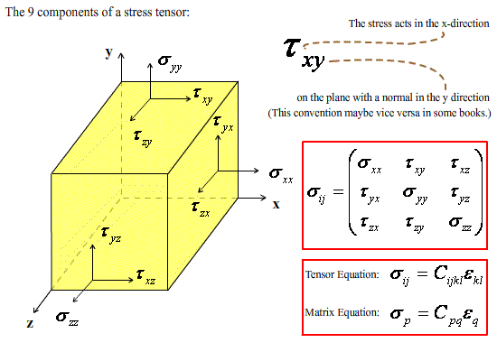
Under off-axis loading of a single lamina the applied stress state can be resolved to give the stresses along the laminar principal axes. The stress state of a body can be described by a stress tensor, shown schematically below, which can be related to the strain tensor by the equation:

\[{\sigma _{ij}} = {C_{ijkl}}{e_{kl}}\;\;\;(11)\]

where C_ijkl is a fourth rank stiffness tensor containing 81 components.

Equation 11 can be rearranged to give:

\[{e_{ij}} = {S_{ijkl}}{\sigma _{kl}}\;\;\;(12)\]

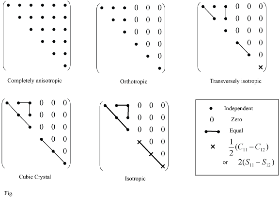
where S_ijkl is the compliance tensor. If the body is in equilibrium both the stress tensor and the stiffness tensor must be symmetric about the diagonal. Then writing Equation 11 as a matrix equation (See Nye 1985) and taking into account the symmetry of the composite itself, the number of independent terms in C_pq reduces to a reasonably small number. A few examples are shown here:

Resolving Stresses within a Lamina

For a single lamina it is reasonable to assume that all the stresses acting are in the laminar plane, so that σ₃ = τ₂₃ = τ₃₁ = 0. Assuming orthotropic symmetry (likely for a lamina) equation 12 becomes

\[\left[ {\begin{array}{*{20}{c}} {{\varepsilon _1}}\\ {{\varepsilon _2}}\\ {{\gamma _{12}}} \end{array}} \right] = {\left[ S \right]^{}}\left[ {\begin{array}{*{20}{c}} {{\sigma _1}}\\ {{\sigma _2}}\\ {{\tau _{12}}} \end{array}} \right] = {\left[ {\begin{array}{*{20}{c}} {{S_{11}}}&{{S_{12}}}&0\\ {{S_{21}}}&{{S_{22}}}&0\\ 0&0&{{S_{66}}} \end{array}} \right]^{}}\left[ {\begin{array}{*{20}{c}} {{\sigma _1}}\\ {{\sigma _2}}\\ {{\tau _{12}}} \end{array}} \right]\;\;\rm{(13)}\]

when stresses are applied along the principal axes of the lamina.

Clearly, when σ₂ = τ₁₂ = 0. \({S_{11}}\) = \(\frac{1}{{{E_1}}}\)

Similar considerations give

\[{S_{22}} = \frac{1}{{{E_2}}},\;\;{S_{66}} = \frac{1}{{{G_{12}}}},\;\;{S_{12}} = \frac{{ - {\nu _{12}}}}{{{E_1}}} = \frac{{ - {\nu _{21}}}}{{{E_2}}}\]

where

\[{\nu _{21}} = \left[ {{f^{}}{\nu _f} + {{(1 - f)}^{}}{\nu _m}} \right]\frac{{{E_2}}}{{{E_1}}}\]

and

ν₁₂ =  [ f ν_f + (1 - f ) ν_m]

Click here for derivation of Poisson's ratio.

We can now find elastic constants for a lamina whose fibres are at an angle θ to the loading direction by the following resolving procedure:

\[\left[ {\begin{array}{*{20}{c}} {{\varepsilon _x}}\\ {{\varepsilon _y}}\\ {{\gamma _{xy}}} \end{array}} \right] = {\left[ {\overline S } \right]^{}}\left[ {\begin{array}{*{20}{c}} {{\sigma _x}}\\ {{\sigma _y}}\\ {{\tau _{xy}}} \end{array}} \right]\;\;(15)\]

The result is that under an arbitrary planar loading system, the transformed compliance tensor replaces the compliance tensor in equation 13. Similar to before,

\[{E_x} = \frac{1}{{{{\overline S }_{22}}}},\;\;{E_y} = \frac{1}{{{{\overline S }_{22}}}},\;\;{G_{xy}} = \frac{1}{{{{\overline S }_{66}}}},\;\;{\nu _{xy}} = - {E_x}{\overline S _{12}},\;\;{\nu _{yx}} = - {E_y}{\overline S _{12}}\]