Mechanics of Fibre-reinforced Composites (all content)

Note: DoITPoMS Teaching and Learning Packages are intended to be used interactively at a computer! This print-friendly version of the TLP is provided for convenience, but does not display all the content of the TLP. For example, any video clips and answers to questions are missing. The formatting (page breaks, etc) of the printed version is unpredictable and highly dependent on your browser.

Contents

Main pages

Additional pages

Aims

On completion of this TLP you should:

• Understand what composites are.
• Understand why composites exhibit high strength and high toughness.
• Be able to calculate the elastic constants for a single lamina and for a laminate.
• Be able to predict the strength of a single lamina and of a laminate.

Before you start

The meanings of some basic elastic constants, including stiffness, strength and toughness.

The use of Ashby Materials Selection Maps ( See the TLP - Optimisation of Materials Properties in Living Systems )

Stress states and Mohr's circle (these are covered in the TLP - Theory of Metal Forming - Stress States and Yielding Criteria )

Tensors and matrices.

Some basic knowledge of plastic deformation and brittle and ductile fracture is also useful.

These are not pre-requisites and it should be possible to make use of this TLP even without knowledge of these concepts.

Introduction

In the search for stiff, light, durable and easily manufactured materials, there has been an ever-increasing emphasis on composites over the past 50 years. Although metals have excellent strength and toughness combinations they are quite dense and many corrode in use. Attention has then turned to ceramics and polymers, which are lighter and more corrosion-resistant, but often lack toughness.

Generally, a composite is a combination of two materials that exhibit desired properties of both constituents, such as compressive strength of the matrix and tensile strength of the fibres. Usually, they consist of ceramic or polymer fibres embedded in a matrix, usually a thermosetting resin such as an epoxy or polyester, but can also be thermoplastics or ceramics or even metals. The fibres are strong due to the removal of flaws in the case of ceramics and molecular alignment for polymers. The three main types of fibre used are:

• Glass
• Carbon
• Aramid (aromatic polyamides, such as Kevlar ).

In some types of composite, the fibres are oriented randomly within a plane, while in others the material is made up of a stack of differently-oriented "plies" to form a laminate, each ply containing an aligned set of parallel fibres.

The choices of composition and of the materials used as matrix and fibre are dependent on the required properties. This can be deduced by deriving a merit index for the performance required followed by the use of Ashby property maps.

As is often the case with science, it is nature that hints at the good mechanical properties of composites, for example wood and bones. For thousands of years we have been using composites, whether it be in brick walls or concrete, and now, composites are widely used in automotive, aerospace, marine and sports applications. Therefore an understanding of how composite materials behave is crucial to any technological advances.

Stiffness of long fibre composites

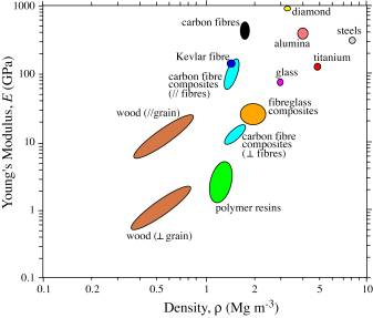
Before we go into the details it is worth noting that the most suitable material for a given application may well not be the stiffest material. For example, for a given force applied to the free end of a cantilevered composite beam, the minimum deflection per unit mass is achieved by maximizing the merit index E / ρ².

Click here for Merit index derivation. (See Optimisation of Materials Properties in Living Systems for more on merit indices)

An Ashby property map (Young's Modulus against Density) for composites:

The axial and transverse Young's Moduli can be predicted using a simple slab model, in which the fibre and matrix are represented by parallel slabs of material, with thicknesses in proportion to their volume fractions, E and (1- E).

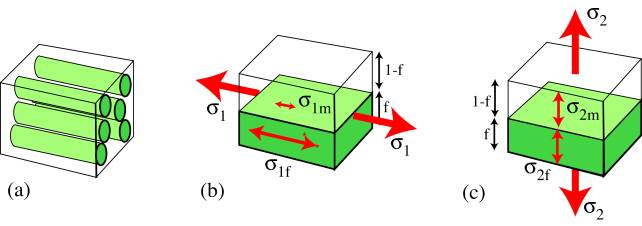
Axial Loading: Voigt model

The fibre strain is equal to the matrix strain: EQUAL STRAIN.

\[{\varepsilon _1} = {\varepsilon _{1{\rm{f}}}} = \frac{{{\sigma _{1{\rm{f}}}}}}{{{E_{\rm{f}}}}} = {\varepsilon _{1{\rm{m}}}} = \frac{{{\sigma _{1{\rm{m}}}}}}{{{E_{\rm{m}}}}} = \frac{{{\sigma _1}}}{{{E_1}}}\]

See definitions of terms

For a composite in which the fibres are much stiffer than the matrix ( E_f >> E_m ), the reinforcement fibre is subject to much higher stresses ( σ_1f >> σ_1m ) than the matrix and there is a redistribution of the load. The overall stress σ₁ can be expressed in terms of the two contributions:

σ₁ = ( 1 - f )σ_1m + f σ_1f

The Young's modulus of the composite can now be written as

\({E_1} = \frac{{{\sigma _1}}}{{{\varepsilon _1}}} = \frac{{\left( {1 - f} \right){\sigma _{1{\rm{m}}}} + f{\sigma _{1{\rm{f}}}}}}{{\left( {\frac{{{\sigma _{1{\rm{f}}}}}}{{{E_{\rm{f}}}}}} \right)}} = \left( {1 - f} \right){E_{\rm{m}}} + f{E_{\rm{f}}}\)   (1)

This is known as the "Rule of Mixtures" and it shows that the axial stiffness is given by a weighted mean of the stiffnesses of the two components, depending only on the volume fraction of fibres.

Transverse Loading: Reuss Model

The stress acting on the reinforcement is equal to the stress acting on the matrix: EQUAL STRESS.

σ₂ = σ_2f = ε_2f E_f = σ_2m = ε_2mE_m

The net strain is the sum of the contributions from the matrix and the fibre:

ε₂ = f ε_2f + ( 1 - f ) ε_2m (5)

from which the composite modulus is given by:

\[{E_2} = \frac{{{\sigma _2}}}{{{\varepsilon _2}}} = \frac{{{\sigma _{2{\rm{f}}}}}}{{f{\varepsilon _{2{\rm{f}}}} + (1 - f){\varepsilon _{2{\rm{m}}}}}} = {\left[ {\frac{f}{{{E_{\rm{f}}}}} + \frac{{(1 - f)}}{{{E_{\rm{m}}}}}} \right]^{ - 1}} \;\;\;\;(6)\]

This "Inverse Rule of Mixtures" is actually a poor approximate for E₂ since in reality regions of the matrix 'in series' with the fibres, close to them and in line along the loading direction, are subjected to a high stress similar to that carried by the reinforcement fibres; whereas the regions of the matrix 'in parallel' with the fibres (adjacent laterally) are constrained to have the same strain as the fibres and carry a low stress. This leads to non-uniform distributions of stress and strain during transverse loading, which means that the model is inappropriate. The slab model provides the lower bound for the transverse stiffness.

A more successful estimate is the semi-empirical Halpin-Tsai expression:

\[{E_2} = \frac{{{E_m}(1 + \xi \eta f)}}{{(1 - \eta f)}}\;\;\;\;(3)\]

where \(\eta\) = \(\frac{{(\frac{{{E_f}}}{{{E_m}}} - 1)}}{{(\frac{{{E_f}}}{{{E_m}}} + \xi )}}\)and ξ ≈ 1

An even more powerful, but complex, analytical tool is the Eshelby method (see Hull and Clyne, 1996).

---

Strength of long fibre composites

For a body under the application of an arbitrary stress state the three most important modes of failure are:

1. Axial tensile failure
2. Transverse tensile failure
3. Shear failure.

axial tensile failure	transverse tensile failure	shear failure

Axial Strength

In the simplest scenario, it is assumed that both the matrix and the fibres deform elastically and subsequently undergo brittle fracture. The EQUAL STRAIN condition applies and there are two possible cases:

a) The matrix has the lower failure ( ultimate) strain ( ε_fu > ε_mu )

b) The fibre has the lower failure strain ( ε_fu < ε_mu )

Click here to see the notations used.

Case a):

The composite stress is given by the rule of mixtures σ₁ = f σ _f + (1 - f) σ_m up until the strain reaches ε_mu . Beyond this point the matrix undergoes microcracking and the load is progressively transferred to the fibres as cracking continues. During this stage there is little increase in composite stress with increasing strain. With further crack growth, if the entire load is transferred to the fibres before fibre fracture, then the composite stress, σ₁, becomes fσ_f and the composite failure stress, σ_1u, is simply f σ_fu :

σ_1u = f σ_fu (4)

Alternatively, if the fibres fail before the entire load is transferred onto them the composite strength is just the weighted average of the failure stress of the matrix, σ_mu , and the fibre stress at the onset of matrix cracking, σ_fmu :

σ_1u = f σ_fmu + ( 1 - f ) σ_mu (5)

The variation of σ_1u with f is shown in graph 2.

Case b):

Again, the composite stress is given by the rule of mixtures σ₁ = f σ_f + ( 1- f ) σ_m up until the strain reaches ε_fu when the fibres fail. Beyond this point the load is progressively transferred to the matrix as the fibres fracture into shorter lengths. Assuming that the fibres bear no load when their aspect ratios are below the critical aspect ratio, s_* = σ_f* / 2τ_i* , which is the critical ratio of the fibre length to its diameter below which the fibre cannot undergo any further fracture, then composite failure occurs at an applied stress of ( 1 - f) σ_mu .

σ_1u = ( 1 - f) σ_mu (6)

Alternatively, if the matrix fracture takes place while the fibres are still bearing some load, i.e. the fibre aspect ratio is more than the critical value, then the composite failure stress is the weighted average of the fibre failure stress, σ_fu , and the matrix stress at the onset of fibre fracture, σ_mfu.

σ_1u = f σ_fu + ( 1 - f) σ_mfu (7)

The variation of σ_1u with f is shown in graph 4.

Why is this approach inaccurate?

See Axial strength inaccuracy.

Generally , the fibre volume fractions fall in the range 30% to 70% (ie, > f ') and since it is usually the case that σ_mu << σ_fu , it is evident from graphs 2 and 4 that the fibre strength is dominant in determining the axial strength of long-fibre composites.

∴ σ_1u ∼ fσ_fu for all axial cases.

Transverse Strength

In general, the presence of fibres reduces the transverse strength and the failure strain significantly relative to the unreinforced matrix. This observed tendency is largely due to high local stresses and strains around the fibre / matrix interface due to differences in the Young's Moduli of the two components. However, the transverse strength is also influenced by many other factors and consequently, it is not possible to deduce a simple estimate of σ_2u without making several approximations.

One approach is to treat the fibres in the composite as a set of cylindrical holes in a simple square array. We then consider the case where the reduction in the composite cross-sectional area is maximum and this leads to the following expression for the transverse strength of a composite having a volume fraction f of fibres:

See Transverse strength derivation

Why is this approach inaccurate?

Click here to see Transverse strength inaccuracy.

Shear Strength

Similarly here, we cannot derive a simple expression for the shear strength. There are a total of six combinations of shearing plane and direction that can be grouped into three sets of equivalent pairs, as shown in the diagrams.

Shear directions

τ₂₁ and τ₃₁ are unlikely to occur since these require breaking of the fibres and it is not obvious which of τ₁₂ and τ₃₂ is easier to happen. When considering the stresses on a thin lamina in the 1-2 plane, τ₃₂ is zero and only τ_12u is important. Finite difference methods (beyond the scope of this TLP) were used to deduce the variation of the shear stress concentration factor, K_s , with fibre volume fraction.

Here, we will just take the result of this analysis, without proof, to be:

τ_12u = K_s τ_mu

Where τ_mu is the ultimate matrix shear stress and K_s varies as shown in graph 6. K_s is about 1 unless the fibre volume fraction is very high (> 70%).

τ_12u ≈ τ_mu (9)

 

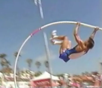
Composite vaulting poles – why don´t they break?

Stresses in a Vaulting Pole

DoITPoMS standard terms of use

Video of a pole vaulter (19 feet 0¼ inches converts to 5.798 m)

DoITPoMS standard terms of use

A composite vaulting pole, of the type shown in the video, typically has a diameter of about 50 mm and the pole is being bent to a radius of curvature, R , of about 1 m. The calculations below show how the peak stress on the outer surface of a 50 % fibre pole can be estimated.

Why are they Strong Enough?

Since σ_1u ~ f σ_fu the strength of the fibres, σ_fu , must therefore be at least about 2 GPa. In fact, the glass fibres used in composites, which are about 7 µm in diameter, have strengths of about 2-3 GPa. Using the Griffith criterion and assuming brittle fracture with a surface energy, γ, of 1 J m ^-2, the maximum flaw size must be less than about 10 nm. The key to their strengths is therefore the absence of large flaws.

Why are they Tough Enough?

It is not immediately clear why the material as a whole should be sufficiently tough, since both constituents are individually very brittle. A repeatedly loaded component will acquire many, relatively large, surface defects, so the fact that it can sustain such high stresses without fracturing indicates that, as a material, the composite has a high toughness. We will explore this in detail in the next section.

Toughness of composites and fibre pull–out

For composites to be useful they not only must be strong, but they must also be tough. The fracture energy, which is related to the fracture toughness by Equation 10, is determined by the available energy absorbing mechanisms.

\[{K_c} = {\sigma _*}\sqrt {\pi c} = \sqrt {E{G_c}} (10)\]

For a composite these are:

• Matrix Deformation
• Fibre Fracture
• Interfacial Debonding and Crack Deflection
• Fibre Pull-Out

Matrix Deformation:

This process is important in ductile matrices, but relatively negligible in brittle matrices. Load transfer onto the fibres reduces the matrix stress and the matrix is unable to deform freely due to the constraint imposed by the fibres. Generally, matrix deformation is unimportant for composites, even in metallic matrices.

Fibre Fracture:

Metallic and polymeric fibres can undergo plastic deformation before fracture (ductile) and this contributes up to a few kJ m ^-2 to the overall fracture energy, whereas brittle fibre fracture only provides a few tens of J m ^-2 . It is important to realize that fibre fracture need not occur in the crack plane. There is a variation in flaw sizes along the fibre and, as a result, there is a variation in strength along the fibre, which can be described by the Weibull Modulus. Typically, fibre fracture in composites makes little contribution to the overall toughness.

Interfacial Debonding and Crack Deflection:

Click here for Interfacial debonding derivation.

G_cd = f s  G_ic

A composite made from brittle constituents can have a surprisingly high toughness if a crack is repeatedly deflected at fibre/matrix interfaces. The work of debonding per unit crack area, G_cd , itself is relatively small, but it allows fibre pull-out, which can potentially contribute significantly to the toughness, to occur.

Example: s = 50, f = 0.5, G_ic = 10 J m ^-2 → G _cd = 0.25 kJ m ^-2

iv) Fibre Pull-out:

The main energy-absorbing mechanism raising the toughness of fibre composites is the pulling of fibres out of their sockets in the matrix during crack advance. This is allowed to take place after interfacial debonding and fibre fracture away from the crack plane have occurred beforehand. The pull-out work per unit crack area is given by:

Click here for Fibre pullout derivation.

G_cp = 4 f s² r τ_i*

Example: s = 50, f = 0.5, r = 10 μm, τ_i* = 20 Mpa →  G_cp = 1.0 MJ m^-2

It is because of these mechanisms that composites exhibit R-curve behaviour.

Off–axis loading of a lamina

Under off-axis loading of a single lamina the applied stress state can be resolved to give the stresses along the laminar principal axes. The stress state of a body can be described by a stress tensor, shown schematically below, which can be related to the strain tensor by the equation:

\[{\sigma _{ij}} = {C_{ijkl}}{e_{kl}}\;\;\;(11)\]

where C_ijkl is a fourth rank stiffness tensor containing 81 components.

Equation 11 can be rearranged to give:

\[{e_{ij}} = {S_{ijkl}}{\sigma _{kl}}\;\;\;(12)\]

where S_ijkl is the compliance tensor. If the body is in equilibrium both the stress tensor and the stiffness tensor must be symmetric about the diagonal. Then writing Equation 11 as a matrix equation (See Nye 1985) and taking into account the symmetry of the composite itself, the number of independent terms in C_pq reduces to a reasonably small number. A few examples are shown here:

Resolving Stresses within a Lamina

For a single lamina it is reasonable to assume that all the stresses acting are in the laminar plane, so that σ₃ = τ₂₃ = τ₃₁ = 0. Assuming orthotropic symmetry (likely for a lamina) equation 12 becomes

\[\left[ {\begin{array}{*{20}{c}} {{\varepsilon _1}}\\ {{\varepsilon _2}}\\ {{\gamma _{12}}} \end{array}} \right] = {\left[ S \right]^{}}\left[ {\begin{array}{*{20}{c}} {{\sigma _1}}\\ {{\sigma _2}}\\ {{\tau _{12}}} \end{array}} \right] = {\left[ {\begin{array}{*{20}{c}} {{S_{11}}}&{{S_{12}}}&0\\ {{S_{21}}}&{{S_{22}}}&0\\ 0&0&{{S_{66}}} \end{array}} \right]^{}}\left[ {\begin{array}{*{20}{c}} {{\sigma _1}}\\ {{\sigma _2}}\\ {{\tau _{12}}} \end{array}} \right]\;\;\rm{(13)}\]

when stresses are applied along the principal axes of the lamina.

Clearly, when σ₂ = τ₁₂ = 0. \({S_{11}}\) = \(\frac{1}{{{E_1}}}\)

Similar considerations give

\[{S_{22}} = \frac{1}{{{E_2}}},\;\;{S_{66}} = \frac{1}{{{G_{12}}}},\;\;{S_{12}} = \frac{{ - {\nu _{12}}}}{{{E_1}}} = \frac{{ - {\nu _{21}}}}{{{E_2}}}\]

where

\[{\nu _{21}} = \left[ {{f^{}}{\nu _f} + {{(1 - f)}^{}}{\nu _m}} \right]\frac{{{E_2}}}{{{E_1}}}\]

and

ν₁₂ =  [ f ν_f + (1 - f ) ν_m]

Click here for derivation of Poisson's ratio.

We can now find elastic constants for a lamina whose fibres are at an angle θ to the loading direction by the following resolving procedure:

\[\left[ {\begin{array}{*{20}{c}} {{\varepsilon _x}}\\ {{\varepsilon _y}}\\ {{\gamma _{xy}}} \end{array}} \right] = {\left[ {\overline S } \right]^{}}\left[ {\begin{array}{*{20}{c}} {{\sigma _x}}\\ {{\sigma _y}}\\ {{\tau _{xy}}} \end{array}} \right]\;\;(15)\]

The result is that under an arbitrary planar loading system, the transformed compliance tensor replaces the compliance tensor in equation 13. Similar to before,

\[{E_x} = \frac{1}{{{{\overline S }_{22}}}},\;\;{E_y} = \frac{1}{{{{\overline S }_{22}}}},\;\;{G_{xy}} = \frac{1}{{{{\overline S }_{66}}}},\;\;{\nu _{xy}} = - {E_x}{\overline S _{12}},\;\;{\nu _{yx}} = - {E_y}{\overline S _{12}}\]

Stiffness of laminates

Aligned composites are very stiff along the fibre axis, but also very compliant in the transverse direction. Many applications equal stiffness in all directions within a plane and the solution to this is to stack together and bond plies with different fibre directions.

Having established the off-axis elastic constants for a single thin ply, we will now establish those for a stack of plies, a laminate. In this case there is a further complication in that while the fibres in each ply make an angle Φ with the reference x-y axes, the elastic constants of the laminate as a whole will also be affected by the angle Φ that the loading direction makes with the same reference x-y axes. The corresponding stress - strain relationship for a laminate is:

\[\left[ {\begin{array}{*{20}{c}} {{\varepsilon _x}}\\ {{\varepsilon _y}}\\ {{\gamma _{xy}}} \end{array}} \right] = {\left[ {{{\overline S }_g}} \right]^{}}\left[ {\begin{array}{*{20}{c}} {{\sigma _x}}\\ {{\sigma _y}}\\ {{\tau _{xy}}} \end{array}} \right] \;\;\;(16)\]

where the subscript g refers to global.

The average stress in the x-direction of the loading system is given by:

\[{\sigma _{x{,^{}}g}} = \frac{{\sum\limits_{k = 1}^n {({\sigma _{x{,^{}}k}}^{}{t_k})} }}{{\sum\limits_{k = 1}^n {{t_k}} }} = {\overline C _{11{,^{}}g}}^{}{\varepsilon _{x{,^{}}g}} + {\overline C _{12{,^{}}g}}^{}{\varepsilon _{y{,^{}}g}} + {\overline C _{16{,^{}}g}}^{}{\gamma _{xy{,^{}}g}}\] (17)

where t_k is the thickness of the k^th ply. This is simply an expansion of equation 16.

And since the in-plane strains are the same for each ply, the stress in the k^th ply can be written as:

\[{\sigma _{x{,^{}}g}} = {\overline C _{11{,^{}}g}}^{}{\varepsilon _{x{,^{}}g}} + {\overline C _{12{,^{}}g}}^{}{\varepsilon _{y{,^{}}g}} + {\overline C _{16{,^{}}g}}^{}{\gamma _{xy{,^{}}g}}\]

This is an expansion of equation 15 for the k^th ply.

Substituting this into equation 17 and equating the coefficients of ε_x,g , we have:

\[{\overline C _{11,g}} = \frac{{\sum\limits_{k = 1}^n {({{\overline C }_{11,g}}^{}{t_k})} }}{{\sum\limits_{k = 1}^n {{t_k}} }}\]

In this way the other components of the stiffness tensor for the laminate can also be found.

The inverse of the stiffness tensor, the compliance tensor, is often obtained because its relationships with the elastic constants are simpler. Like before,

\[{E_x} = \frac{1}{{{{\overline S }_{11{,^{}}g}}}},\;\;\;{G_{xy}} = \frac{1}{{{{\overline S }_{66{,^{}}g}}}},\;\;\;{\nu _{xy}} = - {E_x}{\overline S _{12{,^{}}g}}^{}\]

Clearly the laminate will exhibit different elastic constants if the loading system were applied at an arbitrary angle, Φ, to the x-y coordinate system. Try constructing your own laminate, using the model below, and calculate the elastic constants for different loading angles.

Tensile–shear interactions and balanced laminates

From equation 15, the 'interaction' terms S₁₆ and S₂₆ are both non-zero and this indicates that, under off-axis loading, normal stresses produce shear strains (as well as normal strains) and shear stresses produce normal strains (as well as shear strains). This tensile-shear interaction is also present in laminates, but does not occur if the loading system is applied along the principal axes of a single isolated lamina, in which case S₁₆ = S₂₆ = 0 as in equation 13.

\[{\eta _{xyx}} = {E_x}{\overline S _{16}}\;\; and\;\;{\eta _{xyy}} = {E_y}{\overline S _{26}}\]

The extent of this tensile-shear interaction is quantified by the parameters η_xyx and η_xyy (Click to open pop-up)

Balanced laminates

Tensile-shear interactions are undesirable as they lead to distortions and local microstructural damage and failure. A laminate whose interaction ratios are zero is said to be 'balanced' . Use the model below to investigate the variation of η_xyx with loading angle.

Out–of–plane stresses and symmetric laminates

So far we have only considered in-plane stresses within a given ply and within the laminate, but when plies are bonded together there are also through-thickness (or coupling) stresses, which are difficult to quantify, between the plies. These arise from the differences in the Poisson contractions of each individual ply and can lead to microstructural damage and distortions of the laminate.

Consider the simple case of a uniaxially loaded cross-ply laminate, shown in the animations below.

The strains of the two plies parallel to the loading direction are equal, but the Poisson contraction, ν₁₂ , for the parallel ply is greater than that for the transverse ply, ν₂₁ (See page on Off-axis loading ). The result of this is that there are coupling stresses that try to deform the flat laminate into the shape shown in animation iii). Extending this to a random stacking sequence, it is clear that the Poisson ratio for a single ply will vary with the fibre direction (See model in Stiffness page) and therefore, coupling stresses are present in a laminate if the plies have different constituents or if the laminae are not aligned.

Symmetric laminates

If the laminate has a mirror plane in the laminar plane, i.e. the laminate is symmetric, the coupling forces cancel out and the distortions are significantly reduced, even though local coupling stresses still exist.

For these reasons balanced symmetric stacking sequences are preferred, but this might not always be possible when performance requirements are taken into account.

Failure of laminates and the Tsai–Hill criterion

Similar to the discussions in the page on Strength of long-fibre composites, the failure of laminae can be understood by the same three failure modes: axial, transverse and shear. A number of failure criteria have been proposed for separate plies subjected to in-plane stress states , with the assumption that coupling stresses are not present. We will introduce two here.

Maximum Stress Criterion

This assumes no interaction between the modes of failure, i.e. the critical stress for one mode is unaffected by the stresses tending to cause the other modes. Failure then occurs when one of these critical values, σ_1u , σ_2u and τ_12u , is reached. These values refer to the laminar principal axes and can be resolved from the applied stress system by using the equation

\[\left[ {\begin{array}{*{20}{c}} {{\sigma _1}}\\ {{\sigma _2}}\\ {{\tau _{12}}} \end{array}} \right] = {\left[ T \right]^{}}\left[ {\begin{array}{*{20}{c}} {{\sigma _x}}\\ {{\sigma _y}}\\ {{\tau _{xy}}} \end{array}} \right]\]

where \[\left[ T \right] = \left[ {\begin{array}{*{20}{c}} {{{\cos }^2}\theta }&{{{\sin }^2}\theta }&{2\cos \theta \sin \theta }\\ {{{\sin }^2}\theta }&{{{\cos }^2}\theta }&{ - 2\cos \theta \sin \theta }\\ { - \cos \theta \sin \theta }&{\cos \theta \sin \theta }&{{{\cos }^2}\theta - {{\sin }^2}\theta } \end{array}} \right]\]

( See page on Off-axis loading )

It follows that under an applied uniaxial tension ( σ_y = τ_xy = 0) the critical values of σ_x for each failure mode are:

\[{\sigma _{xu}} = \frac{{{\sigma _{1u}}}}{{{{\cos }^2}\theta }},\;\;\;{\sigma _{xu}} = \frac{{{\sigma _{2u}}}}{{{{\sin }^2}\theta }},\;\;\;{\sigma _{xu}} = \frac{{{\tau _{12u}}}}{{\sin \theta \cos \theta }}.\]

Tsai-Hill Criterion

Other treatments that take into account the interactions between failure modes are mostly based on modifications of yield criteria for metals (See TLP on Theory of Metal Forming - Stress States and Yielding Criteria ). The most important of these is the Tsai-Hill Criterion, which is an adaptation of the von Mises Criterion.

von Mises Criterion for Metals: ( σ₁ - σ₂ )² + ( σ₂ - σ₃ )² + ( σ₃ - σ₁ )² = 2 σ_Y²

where σ_Y is the metal yield stress.

For in-plane stress states ( σ₃ = 0) this reduces to

\[{\left( {\frac{{{\sigma _1}}}{{{\sigma _Y}}}} \right)^2} + {\left( {\frac{{\sigma {}_2}}{{{\sigma _Y}}}} \right)^2} - \frac{{{\sigma _1}{\sigma _2}}}{{{\sigma ^2}_Y}} = 1\]

This is then modified to take into account the anisotropy of composites and the different failure mechanisms to give the following expression.

\[{\left( {\frac{{{\sigma _1}}}{{{\sigma _{1Y}}}}} \right)^2} + {\left( {\frac{{\sigma {}_2}}{{{\sigma _{2Y}}}}} \right)^2} - \frac{{{\sigma _1}{\sigma _2}}}{{{\sigma ^2}_{1Y}}} - \frac{{{\sigma _1}{\sigma _2}}}{{{\sigma ^2}_{2Y}}} + \frac{{{\sigma _1}{\sigma _2}}}{{{\sigma ^2}_{3Y}}} + {\left( {\frac{{{\tau _{12}}}}{{{\tau _{12Y}}}}} \right)^2} = 1\]

The metal yield stresses can be regarded as composite failure stresses and since composites are transversely isotropic ( σ_2u = σ_3u ) we arrive at the Tsai-Hill Criterion for composites.

\[{\left( {\frac{{{\sigma _1}}}{{{\sigma _{1u}}}}} \right)^2} + {\left( {\frac{{\sigma {}_2}}{{{\sigma _{2u}}}}} \right)^2} - \frac{{{\sigma _1}{\sigma _2}}}{{{\sigma ^2}_{1u}}} + {\left( {\frac{{{\tau _{12}}}}{{{\tau _{12u}}}}} \right)^2} = 1\]

Below, the Maximum Stress and the Tsai-Hill criteria are used to predict the dependence on the loading angle of the tensile stress required to cause failure of a single lamina.

Failure of Laminates

The above treatments only apply to single isolated plies. So, in order to extend this to laminates, we must obtain the in-plane stresses in each ply of a laminate subjected to an arbitrary in-plane stress state.

From Equation 13 the stress tensor for the k^th ply is related to the strain tensor by:

\[\left[ {\begin{array}{*{20}{c}} {{\sigma _{1k}}}\\ {{\sigma _{2k}}}\\ {{\tau _{12k}}} \end{array}} \right] = {\left[ C \right]_k}^{}\left[ {\begin{array}{*{20}{c}} {{\varepsilon _{1k}}}\\ {{\varepsilon _{2k}}}\\ {{\gamma _{12k}}} \end{array}} \right]\]

The strain tensor of the k^th ply can be resolved from the strain tensor of the laminate by using Equation 14:

\[\left[ {\begin{array}{*{20}{c}} {{\varepsilon _{1k}}}\\ {{\varepsilon _{2k}}}\\ {{\gamma _{12k}}} \end{array}} \right] = {\left[ {T'} \right]_k}^{}\left[ {\begin{array}{*{20}{c}} {{\varepsilon _x}}\\ {{\varepsilon _y}}\\ {{\gamma _{xy}}} \end{array}} \right]\]

Now, from Equation 16, the laminate strain tensor is related to the laminate stress tensor by:

\[\left[ {\begin{array}{*{20}{c}} {{\varepsilon _x}}\\ {{\varepsilon _y}}\\ {{\gamma _{xy}}} \end{array}} \right] = {\left[ {{{\overline S }_L}} \right]^{}}\left[ {\begin{array}{*{20}{c}} {{\sigma _x}}\\ {{\sigma _y}}\\ {{\tau _{xy}}} \end{array}} \right]\]

Combining these three equations gives:

\[\left[ {\begin{array}{*{20}{c}} {{\sigma _{1k}}}\\ {{\sigma _{2k}}}\\ {{\tau _{12k}}} \end{array}} \right] = {\left[ C \right]_k}^{}{\left[ {T'} \right]_k}{\left[ {{{\overline S }_L}} \right]^{}}\left[ {\begin{array}{*{20}{c}} {{\sigma _x}}\\ {{\sigma _y}}\\ {{\tau _{xy}}} \end{array}} \right]\]

An appropriate failure criterion is then applied and the onset of laminate failure is taken to be the point at which one of the plies fail.

Note that the Maximum Stress Criterion suggests possible modes of failure whereas the Tsai-Hill criterion does not.

Summary

In this TLP we have looked at the approaches taken to go about deriving the in-plane, on-axis elastic constants, in particular the axial and transverse Young's Moduli and the Poisson's ratios , for a composite. From these, we went onto consider the strengths and failure modes of fibre-aligned composites and explore the question as to why they exhibit high strength and toughness , even though the constituent materials tend to be brittle.

With this basic understanding we were able to extend our consideration to laminates , which have a possible advantage of being isotropic, and we have seen how to calculate the elastic constants for an arbitrary in-plane stress state. Off-axis loading presents us with the problem of tensile-shear interactions and coupling stresses in laminates, as a result of which balanced symmetric laminates are preferred. Then in the last section we applied the Maximum Stress Criterion and the Tsai-Hill Criterion to predict the required stress state for laminate failure.

The greatest advantage of composite materials is strength and stiffness combined with lightness and durability; and these properties are the reasons why composites are used in a wide variety of applications.

Questions

Quick questions

You should be able to answer these questions without too much difficulty after studying this TLP. If not, then you should go through it again!

1. In mechanical loading experiments, involving large stresses and long durations, to measure the transverse stiffness of a composite, the experimental values are sometimes lower than the Halpin-Tsai prediction (some even lower than the Equal stress calculation.) Why might this be?

   	a	The matrix deforms plastically during loading.
   	b	The stress distribution is uniform within the composite.
   	c	The strain distribution is uniform within the composite.
   	d	The matrix stiffness is greater than that for fibre.

2. How would you determine the total energy absorbed during fracture of a composite from its stress strain curve? (multiple choice)

   	a	The area under the plot
   	b	The area under the plot times the volume of the composite
   	c	The area under the plot times the mass of the composite
   	d	The gradient of the linear region of the curve.

3. What is the most significant energy absorbing mechanism during composite failure?

   	a	Matrix deformation (this occurs to an even smaller extent than in unreinforced matrices)
   	b	Fibre Fracture (some plastic deformation for ductile fibres, but this is a small contribution to the overall toughness.)
   	c	Crack deflection and interfacial debonding (this is a small contribution, but it allows Fibre pull-out to occur)
   	d	Fibre Pull-out

4. What is the combined work done per unit crack area required for crack deflection and fibre pull-out in a 60 % long-fibre composite? (Data: τ_i* = 40 MPa, G_ic = 8 J m^-2 , fibre radius r = 7 μm, pull-out length x₀ = 840 μm.)

   	a	1.1 MJ m-2
   	b	1.8 MJ m-2
   	c	2.4 MJ m-2
   	d	3.2 MJ m-2

Deeper questions

The following questions require some thought and reaching the answer may require you to think beyond the contents of this TLP.

5. For a laminate made up of 50% volume fraction carbon HS fibres and Nylon 6,6 matrix with a stacking sequence of 0 / 15 /50 / 55 / 60, at what loading angle is the Poisson contraction the minimum?

   	a	10
   	b	30
   	c	50
   	d	90

6. How would you describe a laminate, composed of two constituents, with a stacking sequence of 0/45/80/45/0 subjected to a uniaxial tensile stress at a loading angle of 20 degrees?

   	a	Balanced Symmetric
   	b	Balanced Asymmetric
   	c	Unbalanced Symmetric
   	d	Unbalanced Asymmetric

7. What is the axial stiffness of a long-fibre composite composed of glass fibres arranged in a hexagonal array in an epoxy matrix ? (Data: Glass fibre: E_f = 76 , fibre radius = 3.9 μm, spacing between centres of adjacent fibres = 8 μm Epoxy: E_m = 5 GPa.)

   	a	13 GPa
   	b	21 GPa
   	c	54 GPa
   	d	67 GPa

8. Calculate the axial failure stress for a composite composed of 30% borosilicate glass matrix and 70 % kevlar fibre, assuming that if one of the components fails the entire applied load is transferred to the other component.

   Data: Kevlar fibre: σ_fu = 3.0 GPa, E_f = 130 GPa.
   Borosilicate glass matrix: σ_mu = 0.10GPa, E_m = 64 GPa

   What further assumptions do you need to make?

   	a	0.10 GPa
   	b	1.7 GPa
   	c	2.1 GPa
   	d	<3 GPa

Going further

Books

Hull D. and Clyne T.W. An Introduction to Composite Materials, CUP 1996

Clyne T.W. and Withers P.J. An Introduction to Metal Matrix Composites Materials, CUP, 1993

Piggott M.R. Load Bearing Fibre Composites, Pergamon Press 1980

Chawla K.K. Ceramic Matrix Composites, Chapman and Hall 1993

Chou T.W. Microstructural Design of Fibre Composites, CUP, 1992

Harris B. Engineering Composite Materials, Institute of Metals 1986

Kelly A. Concise Encyclopedia of Composite Materials, Pergamon Press 1994

Ashby M.F. Materials Selection in Mechanical Design, Pergamon Press, 2nd ed. 1999

Nye J. F. Physical Properties of Crystals-Their representation by Tensors and Matrices. Clarendon: Oxford, 1985

Websites

National Composites Network

National Composites Centre

---

Definitions

σ₁ = Axial stress on a composite

σ₂ = Transverse stress on a composite

σ_1f = Axial stress acting on the fibre part of the composite

σ_1m = Axial stress acting on the matrix part of the composite

ε;_1m = Axial strain of matrix part of a composite

ε_1m = Axial strain of matrix part of a composite

E_m = Stiffness of matrix

E_f =  Stiffness of fibre

Merit index derivation

Say the beam is of length L and has a square cross section with sides H, and the applied force has magnitude F

The deflection, δ, of the end of the beam is: \[\delta = \frac{{FL}}{{3EI}}\]

I is the second moment of area of the beam and is given by:\[I = \frac{{{H^4}}}{{12}}\]

 \[∴\;\;\delta = \frac{{4F{L^3}}}{{E{H^4}}}\]

Now the mass of the beam is given by m = L H² ρ

 \[∴\;\;\delta = \frac{{4F{L^5}{\rho ^2}}}{{{m^2}E}}\]

Therefore, in order to minimise δ, we must maximise E/ρ²

Axial strength inaccuracy

It is important to keep in mind that the treatments applied are gross simplifications of reality and are only applicable to brittle composites, e.g. thermosetting polymers and ceramics. In reality, for brittle materials, the load is never entirely transferred to the matrix or to the fibre due to load transfer across interfaces even after fibre or matrix failure. The fibre strength, sfu, is also not a constant for a given type of fibre; instead there is a range of strengths, described by Weibull statistics, due to varying flaw sizes (fracture obeys the Griffith criterion). Another effect not accounted for is the redistribution of stress associated with the fracture of each fibre segments.

Several models have been proposed to treat this process, essentially falling into two groups: “cumulative weakening models” and “fibre break propagation models”.

These are not covered in this TLP (see Hull and Clyne, 1996).

Transverse strength inaccuracy

This is because even the presence of completely debonded fibres would lead to a different stress distribution. Nevertheless, it can be seen from the graph 5 below that this model has a good agreement with experimental data.

Transverse strength derivation

Quick proof

End-on view	Side-on view
Fibre volume fraction = f = π;r2L / 4R2L = πr2 / 4R2	Maximum fibre cross-sectional area fraction  = 2r L / 2R L = \(2\)\( \sqrt{\frac{f}{\pi }} \)  = maximum fractional reduction in cross-sectional area

Minimum matrix cross-sectional area fraction = X = 1 – \(2\)\( \sqrt{\frac{f}{\pi }} \)

The composite ultimate transverse tensile stress is therefore a fraction X of the matrix ultimate tensile stress:

\[{\sigma _{2u}} = {\sigma _{mu}}\left[ {1 - 2{{\left( {\frac{f}{\pi }} \right)}^{1/2}}} \right]\]

Interfacial debonding

Quick proof

We need to start by considering short fibre composites as shown in the diagram above. The work done when a single fibre undergoes interfacial debonding is:

ΔW = 2 π r x₀ G_ic

Now we can sum this over all the fibres intersected by a unit area of the crack to find the work of debonding of the composite per unit crack area, G_cd. If there are N fibres per m² where N is given by

\[N = \frac{f}{{\pi {r^2}_{^{}}}},\]

then there are ( N dx₀ / L ) fibres per m² with an embedded length between x₀ and ( x₀ + dx₀ ).

\[{G_{cd}} = \int\limits_0^L {2\pi r{x_0}{G_{ic}}\frac{{Nd{x_0}}}{L}} \]

Integration gives: G_cd = f s G_ic

This formula only applies to short fibre composites since fibre fracture does not occur if the fibre aspect ratio is less than the critical fibre aspect ratio, s* = σ f* / 2τ i*. (refer to TLP on short fibre composites, which does not exist yet). For long fibre composites there is a small probability that fibre fracture will occur away from the crack plane and debonding will not occur over the whole length of the fibre. In this case G>_cd gives an idea of the magnitude of the energy absorbed.

Single fibre pull out

Quick proof:

Consider a fibre with a remaining embedded length of x being pulled out an increment of distance dx.  The work done is given by the product of the force acting on the fibre and the distance moved in the direction of the force

dW = ( 2 π r x ) τ_i* dx

The work done in pulling this fibre out completely is therefore given by

\[\Delta W = \int\limits_0^{{x_0}} {} 2\pi rx{\tau _{i*}}{\rm{d}}x = \pi rx_0^2{\tau _{i*}}\]

The number of fibres per unit cross-sectional area, N, is related to the fibre volume fraction, f, and the fibre radius, r by

\[N = \frac{f}{{\pi {r^2}}}\]     

so the pull-out work of fracture per unit crack area, G_cp, is given by

\[{G_{{\rm{cp}}}} = N\Delta W = \frac{{f\pi rx_0^2{\tau _{i*}}}}{{\pi {r^2}}} = 4f {s^2} r {\tau _{i*}}\]

Interfacial debonding

Quick proof

We need to start by considering short fibre composites as shown in the diagram above. The work done when a single fibre undergoes interfacial debonding is:

ΔW = 2 π r x₀ G_ic

Now we can sum this over all the fibres intersected by a unit area of the crack to find the work of debonding of the composite per unit crack area, G_cd. If there are N fibres per m² where N is given by

\[N = \frac{f}{{\pi {r^2}_{^{}}}},\]

then there are ( N dx₀ / L ) fibres per m² with an embedded length between x₀ and ( x₀ + dx₀ ).

\[{G_{cd}} = \int\limits_0^L {2\pi r{x_0}{G_{ic}}\frac{{Nd{x_0}}}{L}} \]

Integration gives: G_cd = f s G_ic

This formula only applies to short fibre composites since fibre fracture does not occur if the fibre aspect ratio is less than the critical fibre aspect ratio, s* = σ f* / 2τ i*. (refer to TLP on short fibre composites, which does not exist yet). For long fibre composites there is a small probability that fibre fracture will occur away from the crack plane and debonding will not occur over the whole length of the fibre. In this case G>_cd gives an idea of the magnitude of the energy absorbed.

Poisson’s ratio derivation

The Poisson’s ratio ν_ij describes the contraction in the j-direction due to a stress in the i-direction.

\[{\nu _{ij}} = \frac{{ - {\varepsilon _j}}}{{{\varepsilon _i}}}\]

For a transversely isotropic material such as a composite the following relationship exists:

\[\frac{{{\nu _{12}}}}{{{E_1}}} = \frac{{{\nu _{21}}}}{{{E_2}}}\]

For a composite under axial tension the Poisson strains for the two constituents are:

\[{\varepsilon _{2f}} = - {\nu _f}{\varepsilon _{1f}} = - {\nu _f}\frac{{{\sigma _{1f}}}}{{{E_f}}}\]

\[{\varepsilon _{2m}} = - {\nu _m}{\varepsilon _{1m}} = - {\nu _m}\frac{{{\sigma _{1m}}}}{{{E_m}}}\]

The total transverse strain is simply the weighted sum of the two Poisson strains:

\[{\varepsilon _2} = - \left[ {f{\nu _f}\frac{{{\sigma _{1f}}}}{{{E_f}}} + \frac{{(1 - f){\nu _m}{\sigma _{1m}}}}{{{E_m}}}} \right]\]

Under axial loading the equal axial strain condition applies.

\[∴\;{\varepsilon _2} = - \left[ {f{\nu _f}{\varepsilon _1} + (1 - f){\nu _m}{\varepsilon _1}} \right]\]

\[{\nu _{12}} = - \frac{{{\varepsilon _2}}}{{{\varepsilon _1}}} = {f^{}}{\nu _f} + {(1 - f)^{}}{\nu _m} \;\;\rm{and}\;\;{\nu _{21}} = - \frac{{{\varepsilon _1}}}{{{\varepsilon _2}}} = \left[ {{f^{}}{\nu _f} + {{(1 - f)}^{}}{\nu _m}} \right]\frac{{{E_2}}}{{{E_1}}}\]

Notations

ε_mu is the ultimate failure strain of the matrix.

We have not used 'f' as a suffix for failure to avoid confusion with 'f' for fibre.

σ_mu  is the matrix failure stress.

σ_fmu is the stress in the fibre at the onset of matrix failure.

σ_mfu  is the stress in the matrix when the fibres start to fracture.

---

Academic consultant: Bill Clyne (University of Cambridge)
Content development: Joey Kiatlertpongsa and David Brook
Photography and video: Brian Barber and Carol Best
Web development: David Brook and Lianne Sallows

This DoITPoMS TLP was funded by the UK Centre for Materials Education, the Department of Materials Science and Metallurgy, University of Cambridge, with additional support from the Worshipful Company of Armourers and Brasiers'.