Stiffness of long fibre composites
Before we go into the details it is worth noting that the most suitable material for a given application may well not be the stiffest material. For example, for a given force applied to the free end of a cantilevered composite beam, the minimum deflection per unit mass is achieved by maximizing the merit index E / ρ2.
Click here for Merit index derivation. (See Optimisation of Materials Properties in Living Systems for more on merit indices)
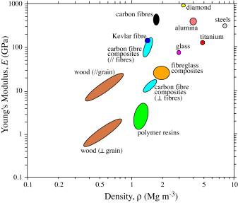
An Ashby property map (Young's Modulus against Density) for composites:
The axial and transverse Young's Moduli can be predicted using a simple slab model, in which the fibre and matrix are represented by parallel slabs of material, with thicknesses in proportion to their volume fractions, E and (1- E).
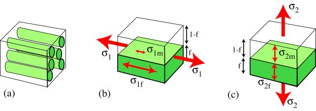
Axial Loading: Voigt model
The fibre strain is equal to the matrix strain: EQUAL STRAIN.
\[{\varepsilon _1} = {\varepsilon _{1{\rm{f}}}} = \frac{{{\sigma _{1{\rm{f}}}}}}{{{E_{\rm{f}}}}} = {\varepsilon _{1{\rm{m}}}} = \frac{{{\sigma _{1{\rm{m}}}}}}{{{E_{\rm{m}}}}} = \frac{{{\sigma _1}}}{{{E_1}}}\]
See definitions of terms
For a composite in which the fibres are much stiffer than the matrix ( Ef >> Em ), the reinforcement fibre is subject to much higher stresses ( σ1f >> σ1m ) than the matrix and there is a redistribution of the load. The overall stress σ1 can be expressed in terms of the two contributions:
σ1 = ( 1 - f )σ1m + f σ1f
The Young's modulus of the composite can now be written as
\({E_1} = \frac{{{\sigma _1}}}{{{\varepsilon _1}}} = \frac{{\left( {1 - f} \right){\sigma _{1{\rm{m}}}} + f{\sigma _{1{\rm{f}}}}}}{{\left( {\frac{{{\sigma _{1{\rm{f}}}}}}{{{E_{\rm{f}}}}}} \right)}} = \left( {1 - f} \right){E_{\rm{m}}} + f{E_{\rm{f}}}\) (1)
This is known as the "Rule of Mixtures" and it shows that the axial stiffness is given by a weighted mean of the stiffnesses of the two components, depending only on the volume fraction of fibres.
Transverse Loading: Reuss Model
The stress acting on the reinforcement is equal to the stress acting on the matrix: EQUAL STRESS.
σ2 = σ2f = ε2f Ef = σ2m = ε2mEm
The net strain is the sum of the contributions from the matrix and the fibre:
ε2 = f ε2f + ( 1 - f ) ε2m (5)
from which the composite modulus is given by:
\[{E_2} = \frac{{{\sigma _2}}}{{{\varepsilon _2}}} = \frac{{{\sigma _{2{\rm{f}}}}}}{{f{\varepsilon _{2{\rm{f}}}} + (1 - f){\varepsilon _{2{\rm{m}}}}}} = {\left[ {\frac{f}{{{E_{\rm{f}}}}} + \frac{{(1 - f)}}{{{E_{\rm{m}}}}}} \right]^{ - 1}} \;\;\;\;(6)\]
This "Inverse Rule of Mixtures" is actually a poor approximate for E2 since in reality regions of the matrix 'in series' with the fibres, close to them and in line along the loading direction, are subjected to a high stress similar to that carried by the reinforcement fibres; whereas the regions of the matrix 'in parallel' with the fibres (adjacent laterally) are constrained to have the same strain as the fibres and carry a low stress. This leads to non-uniform distributions of stress and strain during transverse loading, which means that the model is inappropriate. The slab model provides the lower bound for the transverse stiffness.
A more successful estimate is the semi-empirical Halpin-Tsai expression:
\[{E_2} = \frac{{{E_m}(1 + \xi \eta f)}}{{(1 - \eta f)}}\;\;\;\;(3)\]
where \(\eta\) = \(\frac{{(\frac{{{E_f}}}{{{E_m}}} - 1)}}{{(\frac{{{E_f}}}{{{E_m}}} + \xi )}}\)and ξ ≈ 1
An even more powerful, but complex, analytical tool is the Eshelby method (see Hull and Clyne, 1996).