Brittle Fracture (all content)
Note: DoITPoMS Teaching and Learning Packages are intended to be used interactively at a computer! This print-friendly version of the TLP is provided for convenience, but does not display all the content of the TLP. For example, any video clips and answers to questions are missing. The formatting (page breaks, etc) of the printed version is unpredictable and highly dependent on your browser.
Contents
Main pages
Additional pages
Aims
On completion of this TLP you should understand:
- that materials break by cracking;
- what determines whether a material will crack or not;
- what determines whether cracking is catastrophic or more gradual;
- the concepts of the fracture energy, strain energy release rate, fracture toughness and stress intensity factor.
Before you start
You need not do it now, but you may want to look at the TLP on photoelasticity.
Introduction
The consequences of something breaking can be a pest, or utterly disastrous, as when the pedal drops off one’s bike, but without it, biting and crunching, breaking into crisp packets, pulverizing coal, oil drilling and many other processes would be impossible. The most dramatic failures are catastrophic, but sometimes they can be very gradual even in the most brittle materials.
Here we discuss what determines when a material will break, and whether failure will be catastrophic or more gradual. We show cracking is controlled by the energy changes that occur - it is not the stress at the crack tip that is important..
The emphasis here is on brittle fracture, and although all of this is relevant to metals, we do not discuss the details of ductile fracture.
When do atomic bonds break?
Fracture is the separation of atoms. We normally do this by applying a force to the body. How big a force should we need?
We want to know how the energy, U, changes with distance, r, between two atoms. A commonly used expression (known as the Lennard-Jones potential is
$$U(r) = 4\varepsilon \left[ {\left( {{{{\beta ^{12}}} \over {{r^{12}}}}} \right) - \left( {{{{\beta ^6}} \over {{r^6}}}} \right)} \right]$$
Other potentials exist, but the argument is essentially the same.
This contains a short range repulsive term, and a long range attractive term. The parameter ε is a measure of the depth of the potential well, and β is the non-infinite distance where the interparticle potential equals zero.
Use the animation to see how the energy changes as the distance between two atoms is varied.
The force between a pair of atoms is calculated by taking the derivative of the energy function, giving:
$$F = {{{\rm{d}}U{\rm{(r)}}} \over {{\rm{d}}r}} = 24\varepsilon \left[ { - 2\left( {{{{\beta ^{12}}} \over {{r^{13}}}}} \right) + \left( {{{{\beta ^6}} \over {{r^7}}}} \right)} \right]$$
Now see how the force between the atoms changes with distance. What is the force needed to separate the atoms in a crystal?
Because we are interested in the material’s properties we normally think of failure stresses, so in a unit area of crystal we need to know how many bonds in an area of crystal normal to the applied force are carrying the load, say 6.25 × 10⁻²² m2.
From the animation it is clear that materials should have breaking stresses of the order of 10 GPa, but a piece of glass normally breaks at a stress of 70 MPa.
Where have we gone wrong?
What have we just estimated? It is the stress required to break the bonds on a given plane simultaneously, what becomes the fracture surface. So do all the bonds on a given plane break at once?
Anybody who has opened a packet of crisps or torn a sheet of paper knows the answer is ‘no’ – the bonds break a few at a time – at the tip of a growing crack.
So the analysis above does not describe what actually happens when a material breaks, which is a relief as the predictions were no good anyway.
Why do cracks weaken a material?
Let’s watch a crack grow. We’ve used paper here, because the loads are low and we’ve applied a force to the paper sheet by stretching it across a metal strip in bending, as shown in the video.
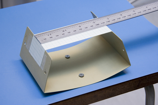
Loading situation of a strip of graph paper.
Video of paper tearing at a preformed crack
You can see that initially the paper is quite capable of withstanding the stress applied to it by the loading jig. And this is fine even when there is quite a big cut in it. But when the cut is lengthened the crack grows quite suddenly.
Is the effect simply one of decreasing the intact section area, causing an increase in stress on the intact section?
Effect of cracks – reducing the intact cross-section
Strips of paper 200 mm long and 70 mm wide were cut. Some had notches cut into one side giving a reduction in the intact cross-section of 5.16 × 10⁻⁶ m2. These and strips without notches were stretched until they broke in a tensile test machine.
The average stress required to break the strip without a notch was measured to be 19.3 MPa.
Where the intact cross-section was reduced by a factor of 1.14 the average breaking stress was measured as 9.4 MPa.
So the breaking strength falls by a greater factor than the reduction in cross-sectional area.
This is why cracks are so dangerous – because they weaken the material more than you would expect from the reduction in intact cross-section. Why?
Inglis and the crack tip stress idea
In 1913, Inglis calculated what the stresses and strains were in an elastic plate containing an elliptical crack, with semi-axes b and c, and under an applied stress σ - applied vertically in this case.
He found that the stress at the crack tip, σt , was given by
$${\sigma _{\rm{t}}} = \sigma {\rm{ }}\left( {1 + 2{c \over b}} \right)$$
For a sharp crack, i.e. c >> b, the stress would be much greater at the crack tip So failure could occur by cracking because it’s only at a crack tip that the stress required to break a bond, or simultaneously break a given number of bonds in a unit area of material, is reached.
So far, so good, but σt depends on the SHAPE of the crack, i.e. c / b – and we know that the length is important.
By looking at crack tip stress fields using photoelasticity, we can see that stresses are indeed concentrated at crack tips. Inglis was correct about this.
It's the idea that a critical stress to break a bond is needed that is wrong.
Can we calculate the energy changes?
In the beginning, we calculated the force, and hence the stress, for failure by considering the energy changes as the atoms moved apart.
Why not consider cracks like this?
The first person to do this was A.A. Griffith in 1920. He considered a body in tension, but tension is rather complicated, so let’s consider another stress-state – wedging.
Wedging is what you do when you split a piece of wood, or try to peel paper off the wall by getting your fingernail underneath it. It’s shown in the animation where a block of thickness h, is being driven in under a layer of thickness d.
So why does the energy, U, of the body change with crack length?
From the animation you can see there are 3 contributions:
Pushing the wedge in causes the peeling layer to bend more, increasing the strain energy, UE. And only the layer between the crack tip and the point where the layer touches the wedge is bending. Using the TLP on beam bending (a more detailed derivation can be found here) gives UE as
$${U_{\rm{E}}} = {{E{d^3}{h^2}} \over {8{c^3}}}$$
What the about work done by the applied force, UF?
We can see that the action of the wedge is the same as a force applied at the point where the wedge touches the peeling ligament. So as the crack grows the force moves sideways, i.e. perpendicular to its line of action, so no work is done. So
UF = 0
Finally, as the crack length changes, the energy of the surfaces, US, changes, giving
US = c R,
where R is known as the fracture energy, the energy required to create new surfaces.
The total energy, U, of the body is just these 3 terms added up.
So what does this have to do with cracking?
Again explore the animation above and start with the default values.
What will be the crack length, c*, where the body has the lowest energy? We can find c* by differentiating the expression for u with respect to c and setting dU / dc = 0.
What will happen if the crack is shorter than this?
The energy of the body would increase if c < c*, so the crack would grow until c = c*, and then stop.
This is called stable cracking – it happens where there is a stable equilibrium in the energy change with crack length.
But what happens if the initial crack length is longer than the equilibrium value, or if we pull the wedge out?
What is predicted?
What happens if the wedge is pulled out?
If we pull the wedge out, the crack length should decrease; in other words, the crack should heal. To test this, Obreimoff cleaved crystals of muscovite mica by wedging. On pushing the wedge in he found that the crack grew at a constant distance ahead of the crack tip, as predicted, and estimated a value of R for mica close to that measured elsewhere.
Then he pulled the wedge out. His first tests in air showed no crack healing.
Then he tried testing in vacuum – healing really did occur.
Obreimoff thought that this occurred because in air chemical groups attached themselves to the fresh mica surfaces, just as fluff sticks on a toffee in your pocket, so that the surfaces no longer stick.
This showed cracking really was thermodynamic in nature – totally different from the critical stress ideas.
This reversibility, crack healing, seems a strange idea at first. But we know surfaces stick together – that is the cause of friction – and there have been many observations of this on metal sheets, on probes in atomic force microscopes. And it is what we would expect if we think of a surface in terms of unfulfilled chemical bonds, desperate for other electrons.
What about tension?
It is not as easy to estimate UE for tension. Griffith used Inglis’ analysis for the overall stress and strain fields in a cracked body, under a constant applied load. This gives UE as
$${U_{\rm{E}}} = {{\pi {c^2}{\sigma ^2}} \over E}$$
In other words there is an increase in the elastic strain energy as the crack grows.
However when the crack grows, work is done by the applied force, F, and is equal in magnitude to twice the change in elastic strain energy. (Think of the work done by the applied force and the elastic energy changes on a uniform bar loaded in tension.) As it is work done on the system, the sign is opposite to that of UE, so that
$$ - {U_{\rm{F}}} + {U_{\rm{E}}} = - {{\pi {c^2}{\sigma ^2}} \over E}$$
where UF is the work done by the applied force, UE is the elastic energy change on cracking and US is the work required to create two new surfaces.
The work associated with creating new crack faces, US.
US = 2 c R
where R is the fracture energy.
Combining the terms of this energy expression we obtain:
$$U = - {{\pi {\sigma ^2}{c^2}} \over E} + 2cR$$
The energy function is plotted in the following animation:
How does cracking occur now?
The energy terms above vary with c as shown. Although there is an equilibrium, it is unstable in tension whereas it was stable in wedging.
Adding the energies and differentiating gives the equilibrium crack length ce as
$${c_{\rm{e}}} = {{E{\rm{ }}R} \over {\pi {\sigma ^2}}}$$
Since this is an unstable equilibrium, once it is surpassed, fracture will occur, but will it be catastrophic?
Another way of expressing the energies
What we have been doing so far is to calculate how U varies with c, and then find the equilibrium value of c by differentiating U with respect to c. Looking at the terms they fall into two types:
Those that come from the loading system, UE and UF: let’s add these together and call the sum UM
- These give the driving force for cracking
Those that are associated with the material, US
- This gives the resistance to cracking
Equilibrium will occur when
$${{{\rm{d}}U{\rm{(}}c{\rm{)}}} \over {{\rm{d}}c}} = 0$$
Breaking our energies into the two different types, gives
$$ - {{{\rm{d}}{U_{\rm{M}}}} \over {{\rm{d}}c}} = {{{\rm{d}}{U_{\rm{S}}}} \over {{\rm{d}}c}}$$
From our expression for cracking in tension
$${{{\rm{d}}{U_{\rm{S}}}} \over {{\rm{d}}c}} = 2R$$
and
$${{{\rm{d}}{U_{\rm{M}}}} \over {{\rm{d}}c}} = - {{2\pi {\sigma ^2}} \over E}{\rm{ }}c = 2G$$
where G is the energy per unit area of crack and so is often called the strain energy release rate, or the crack driving force. Now the turning point occurs when
G = R
This is our condition for cracking, that the crack driving force, G, equals the fracture resistance of the material, R.
Another way of calculating the energies
Consider a crack growing from C by an amount δc to C'. Before cracking occurs there are stresses acting ahead of the crack and across the plane C − C'. After crack growth these stresses have been relaxed to zero as the newly created surfaces move from their initial position at u = 0 to form the crack.
If we knew the stresses ahead of the crack and displacements that relaxed them to zero, we could estimate the total mechanical work, δUM, when the crack grows by δc.
What are the displacements, u?
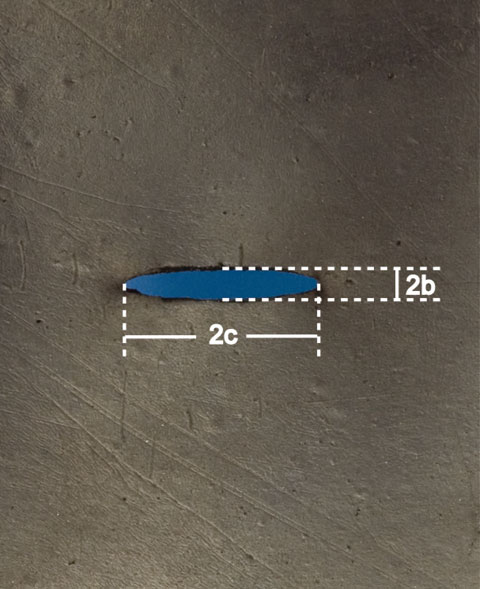
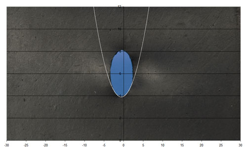
To find these we make a sharp cut in a rubber sheet, something compliant enough to get measurable shape changes without breaking, and stretch it, see below
We can plot the opening of the crack, u, against the distance from the crack-tip, r. Remember r is taken as positive ahead of the growing crack. The opening is therefore at negative values of r. From the picture
u ∝ −r½
where r is the distance from the crack tip, taken as positive in the direction ahead of the growing crack. The crack opening, u, at a given point is therefore at a negative value of r. A full elastic analysis gives
$$u = 4{K \over E}{\left( {{{ - r} \over {2\pi }}} \right)^{{1 \mathord{\left/ {\vphantom {1 2}} \right. \kern 0.1em} 2}}}$$
where K is a constant known as the stress intensity factor and E is the Young modulus.
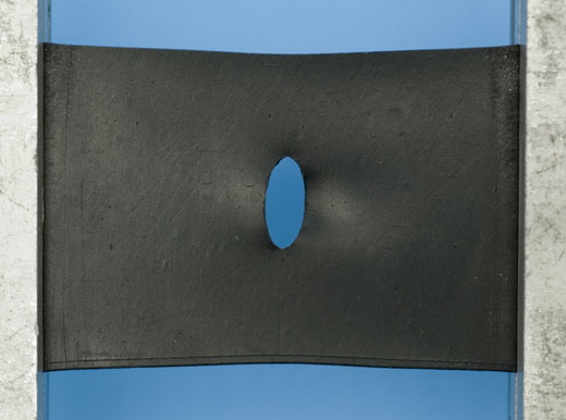
We can see this well by simply stressing a rubber sheet with a cut slit, the shape of the crack being clearly parabolic. A curve with equation
y = m(x − a)2 + c can be fitted to the tip of the curve.
What are the stresses ahead of a crack tip?
If the crack opening is parabolic, it seems not unreasonable to think that the stresses ahead of the crack (not at the crack tip) are too, so
$$\sigma = {K \over {{{\left( {2\pi r} \right)}^{{1 \mathord{\left/ {\vphantom {1 2}} \right. \kern 0.1em} 2}}}}}$$
We can reassure ourselves by carrying out a Finite Element simulation. Taking the expressions for u and σ and as the elastic energy is proportional to σ × u, we can see that the change in mechanical energy, δUM, is likely to be proportional to K2/E. To check we need to integrate δUM over the increment of crack growth δc. See here. As expected, this gives:
$$G = {{{K^2}} \over E}$$
Now, we said cracking occurred when G = R, an equivalent expression is
K = KC
where KC is the critical stress intensity factor at which the crack will grow, known as the fracture toughness. Both criteria are based on the idea that the mechanical energy per increment of crack growth must reach some critical value. Both are entirely equivalent and both calculate the energy changes on cracking.
Why bother if they are the same?
K is useful because stress intensity factors, like stresses, are additive. Irwin showed that any loading state could be broken down into 3 different types of loading that he called modes, I, II and III:
To get the total K, we just sum the contribution from each of the three modes.
This is much more difficult to do with energies, where we would have to think about interaction terms.
Coping with a scatter in strength
The Griffith expression shows that the stress required for failure in tension is dependent on the size of the largest flaw, c, according to \(1/\sqrt c \).
In very brittle materials the flaw sizes cannot be easily measured, so it is sometimes impossible to calculate a minimum strength.
Using a method by Weibull, we can then find the chance of survival of a sample as a function of applied stress. We can then extrapolate back to an acceptable probability of failure and find the corresponding stress.
The linked derivation gives a relationship of
$$\ln \ln {1 \over {{S_n}}} = m\ln \sigma - (m\ln {\sigma _{\rm{o}}} + \ln N)$$
where Sn is the probability of survival, and σ is the fracture stress.
We can treat our results from the tensile of testing of paper with Weibull statistics:
Using Weibull’s method
To determine the survival probability associated with each stress we start by testing some samples, in this case the graph paper used in the first video of the TLP. The following table shows all the collected data, and the calculated values needed:
| n | UTS | Sn | ln ln (1/Sn) | ln σ |
| /MPa | ||||
| 1 | 21.28 | 0.07 | 0.9704 | 16.8733 |
| 2 | 20.86 | 0.14 | 0.6657 | 16.8531 |
| 3 | 20.20 | 0.21 | 0.4321 | 16.8213 |
| 4 | 20.20 | 0.29 | 0.2254 | 16.8211 |
| 5 | 20.12 | 0.36 | 0.0292 | 16.8173 |
| 6 | 19.30 | 0.43 | -0.1657 | 16.7755 |
| 7 | 19.03 | 0.50 | -0.3665 | 16.7615 |
| 8 | 18.87 | 0.57 | -0.5805 | 16.7531 |
| 9 | 18.53 | 0.64 | -0.8168 | 16.7347 |
| 10 | 18.49 | 0.71 | -1.0892 | 16.7330 |
| 11 | 18.11 | 0.79 | -1.4223 | 16.7122 |
| 12 | 18.10 | 0.86 | -1.8698 | 16.7112 |
| 13 | 17.74 | 0.93 | -2.6022 | 16.6912 |
From Weibull treatment of graph paper test.xls
Remember that Sn is the probability of survival at a given stress, given by
$${S_n} = {n \over {{n_{\rm{T}}} + 1}}$$, where nT is the total number of samples and σ is the fracture stress of the sample.
The data has been ordered with the highest strength being 1, and the lowest numbered down to n.
When we plot the graph of ln ln (1/Sn) vs ln (UTS), we get the following:
From Weibull treatment of graph paper test.xls
We can then read off the graph for various values of Sn. For instance if we wanted a 99% chance of survival, we read off from –4.60 on the y axis, which corresponds to 15.1MPa.
A fully interactive version of this spreadsheet and graph tool can be downloaded here.
Simulation of Weibull modulus experiment
In the simulation below it shows an experiment that can be done to see how a material fails in compression and the scatter of loads it requires.
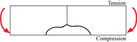
In the simulation above the failure crack was shown to break directly across the material in reality the material is more likely to break in more of a ‘Y’ shape. This phenomenon is known as compression curl or cantilever curl. There is not much quantitative data about why this occurs however this is seen when many materials break.
The rod was loaded in bending, placing the top in compression and the bottom in tension. The crack would have started to grow from the side under tension. However instead of breaking straight through the crack splits and propagates to two points on the compression side creating the characteristic ‘y’ shape fracture. One explanation for this is, that as the crack moves through to the compressive side the stresses cannot be relaxed fast enough, as it is a high speed failure, so the crack can split and take a longer route and this is known as compression curl. The characteristic shape can be useful to identify the side that was in tension in failed samples.
The images below show the results of compression curl on Perspex that was put into uniaxial compression.
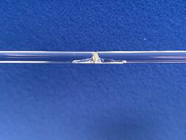
Fracture path in perspex put in uniaxial compression
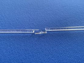
Fracture pieces of perspex after it was put in uniaxial compression
When does the sample fail completely?
It is incorrect to say that failure must occur when
G = R
There will be some cracking but complete failure (as in tension) also requires that
$${{{{\rm{d}}^2}U(c)} \over {{\rm{d}}{c^2}}} < 0$$
i.e. the energy is at a maximum, or
$${{{\rm{d}}G} \over {{\rm{d}}c}} > {{{\rm{d}}R} \over {{\rm{d}}c}}$$
In other words failure will be catastrophic when the rate of increase of the driving force with crack growth is greater than the change in R with crack growth, which we have taken as a constant.
Alternatively cracking will be stable when
$${{{{\rm{d}}^2}U(c)} \over {{\rm{d}}{c^2}}} > 0$$
i.e. the energy is at a minimum, or
$${{{\rm{d}}G} \over {{\rm{d}}c}} < {{{\rm{d}}R} \over {{\rm{d}}c}}$$
That is, as the crack grows, the resistance to cracking, R, increases faster than the driving force, G.
Sub-critical crack growth and R-curves
It is commonly observed that cracks can grow stably in a structure over a period of time. Oddly this phenomenon, known as fatigue, tends to occur in tougher materials. This suggests that toughening does not simply increase the magnitude of the fracture energy but changes the way in which a crack grows.
Consider a material toughened by crack bridging in which intact ligaments across the crack faces are left behind as the crack grows. Toughening occurs because separating the crack faces then requires extra work in order to either stretch the ligament or pull it out of the matrix in which it is embedded. This type of mechanism occurs in many different materials, including:
- rubber toughened polymer
- materials containing either fibres or elongated grains
This animation shows how an R-curve is generated when a crack propagates through a material containing ligaments perpendicular to the direction of crack propagation.
After each critical point, the simulation will pause. It can then be continued by clicking the 'proceed' button.
This type of behaviour is known as R-curve behaviour. We can see that as we load the material containing a small flaw, it will begin to grow (under an increasing applied stress intensity factor) until the process zone is fully developed. The crack in the process zone has a different shape to that outside it because of the forces that due to the intact ligaments. Once the process zone has developed fully then the whole crack will move forward with the process zone size remaining a constant size. As process zones exist in all toughened materials we might expect that they would all show R-curves and this is the case as shown below.
Showing the R-curve due to grain interface bridging in a silicon nitride containing elongated grains and an alumina containing silicon carbide fibres.
Summary
It has been shown that energy arguments describe how cracking occurs, but that there is more than one way of working out the energy changes.
Questions
Quick questions
You should be able to answer these questions without too much difficulty after studying this TLP. If not, then you should go through it again!
-
The Lennard-Jones potential best describes which of the following:
-
Which of the following situations is required for fast fracture to occur?
-
In the wedging setup, which of the following will *not* influence the critical crack length?
-
Which one of Irwin's modes of fracture best describes a car tyre skidding on a dry road?
-
What is the critical stress intensity factor equal to when no residual stresses are present?
-
What best describes the situation in wedging?
Going further
Books
A best overall book on cracking is that by Brian Lawn, Fracture of brittle solids, 1993, Cambridge University Press. You should also look at Molecular adhesion and its applications by Kevin Kendall. For the metalllurgist, the short monograph by Withers & Knott is exceptionally useful.
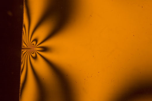
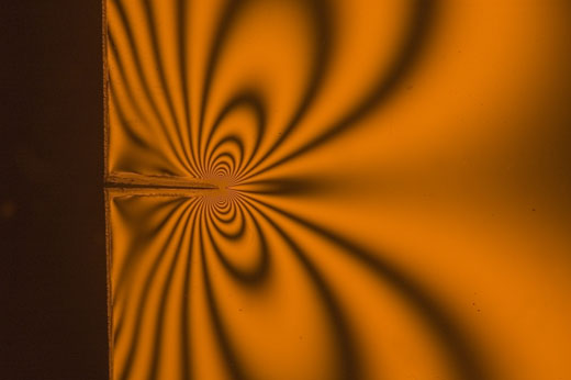
Looking at an induced stress field
Ccrack 0.75 mm long under monochromatic light
Crack 3.1 mm long under monochromatic light
Crack 7.25 mm long under monochromatic light
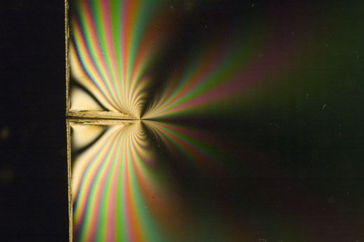
Crack 7.25 mm long under white light
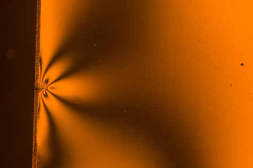
Are stresses concentrated at a crack tip?
A small crack could be made to grow into the material, by gently tapping a razor blade onto the edge of a piece of polycarbonate. This can introduce internal stresses, so the sample was annealed at 140 °C for 45 minutes to reduce them as much as possible.
The sample was loaded so that the crack was perpendicular to the loading direction and viewed under polarised light.
The dark bands show contours of constant difference between the two principal stresses. Away from the crack, zero stress can be assumed parallel to the crack direction. This allows us to calculate a ‘far field’ stress.
We know the stress-optical coefficient for polycarbonate, and the thickness of the sample, so the stress difference for each successive contour can be calculated at just over 2.5 MPa.
The contours become closer together near the crack tip – showing that the stress increases as you get nearer the crack tip. Some more images, including white light and variable crack length pictures can be viewed here.
7.25 mm crack in polycarbonate under monochromatic light
Weibull analysis
The Weibull approach considers a chain of N links. So the survival of the chain under load requires that ALL the links survive.
Pr (survival of CHAIN) = Pr (ALL links survive)
$$\displaylines{ {F_{\rm{C}}} = 1 - {({S_{\rm{L}}})^N} \cr = 1 - {(1 - {F_{\rm{L}}})^N} \cr} $$
What is FL?
$${F_{\rm{L}}} = 1 - \exp - {\left( {{\sigma \over {{\sigma _{\rm{o}}}}}} \right)^m}$$
$${S_{\rm{L}}} = \exp - {\left( {{\sigma \over {{\sigma _{\rm{o}}}}}} \right)^m}$$
$$\displaylines{ {S_{\rm{C}}} = {\left[ {\exp - {{\left( {{\sigma \over {{\sigma _{\rm{o}}}}}} \right)}^m}} \right]^N} \cr = \exp - N{\left( {{\sigma \over {{\sigma _{\rm{o}}}}}} \right)^m} \cr} $$
Taking logarithms
$$\ln {1 \over S} = - N{\left( {{\sigma \over {{\sigma _{\rm{o}}}}}} \right)^m}$$
$$\ln \ln {1 \over S} = m\ln \sigma - (m\ln {\sigma _{\rm{o}}} + \ln N)$$
Estimate of the strain energy in a bent beam
In pure bending, where the moment, M, is constant along a beam of length L, the curvature of the beam, κ, and the angle, θ, through which the beam is bent is given by
$$\kappa = {M \over {EI}}{\rm{, so }}\theta = {M \over {EI}} \cdot L$$
The strain energy, Ustrain, is given by
$${U_{{\rm{strain}}}} = {1 \over 2}M\theta = {{{M^2}L} \over {2EI}}$$
Here the moment therefore varies along the length so that Ustrain becomes
$${U_{{\rm{strain}}}} = \int\limits_0^L {{{{M^2}} \over {2EI}}} {\rm{ d}}x$$
where x is the distance along the beam from the point of application of force at the free end. The bending moment is given at any point x by M = Fx so,
$${U_{{\rm{strain}}}} = {{{F^2}{L^3}} \over {6EI}}$$
The work done, Wforce, by the applied force when the beam is bent is
$${W_{{\rm{force}}}} = {1 \over 2}F\delta $$
This is equal to the strain energy in the beam, Ustrain, so that
$$F = {{3EI\delta } \over {{L^3}}}$$
Substituting for F in the expression for Ustrain and remembering that I = wd3/12 for a beam of thickness d and width w gives
$${U_{{\rm{strain}}}} = \left[ {{{Ew{d^3}{\delta ^2}} \over {8{L^3}}}} \right]$$
For our peeling layer of unit width, i.e. w = 1, then L = c and d = h, so the strain energy in the peeling ligament, UE, is
$${U_{\rm{E}}} = {{E{d^3}{h^2}} \over {8{c^3}}}$$
Finite Element simulation of a sharp crack
A Finite Element simulation was carried out on the same loading setup as the polycarbonate studied previously. A sharp crack was used, i.e. an infinitely small crack tip radius.
The stress perpendicular to the crack plane, σ11, decreases with distance from the crack tip:
This curve can be fitted closely to a r−1/2 curve, showing that our prediction for the stresses ahead of a crack tip is accurate.
The stresses ahead of the crack tip
Consider the stresses acting across the plane in which the crack is growing and ahead of the crack tip. This analysis assumes that the normal stresses on the crack faces are zero and gives the stress ahead of the crack tip as
$$\sigma = {K \over {{{\left( {2\pi r} \right)}^{{1 \mathord{\left/ {\vphantom {1 2}} \right. \kern-0em} 2}}}}}$$
$$\eqalign{ & = \int\limits_{\delta {\rm{c}}}^0 {{K \over {{{\left( {2\pi r} \right)}^{{1 \mathord{\left/ {\vphantom {1 2}} \right. \kern-0em} 2}}}}}} {\rm{ 4 }}{K \over E}{\left( {{{\delta c - r} \over r}} \right)^{{1 \mathord{\left/ {\vphantom {1 2}} \right. \kern-0em} 2}}}{\rm{d}}r \cr & = {2 \over \pi }{{{K^2}} \over E}\int\limits_{\delta {\rm{c}}}^0 {{{\left( {{{\delta c - r} \over r}} \right)}^{{1 \mathord{\left/ {\vphantom {1 2}} \right. \kern-0em} 2}}}{\rm{d}}r} \cr} $$
We can integrate this by substituting for r using the expression
r = δc sin2ω
which gives dr as
dr = 2 δc sinω cosω dω
The limits of integration now become
$$\eqalign{ & r = 0,{\rm{ }}\omega = 0 \cr & r = \delta c,{\rm{ }}\omega = {\pi \over {\rm{2}}} \cr} $$
Integrating,
$${\int\limits_{\delta {\rm{c}}}^0 {\left( {{{\delta c - r} \over r}} \right)} ^{{1 \mathord{\left/
{\vphantom {1 2}} \right.
\kern-0em} 2}}} = \int\limits_{{\pi \mathord{\left/
{\vphantom {\pi 2}} \right.
\kern-0em} 2}}^0 {2{\rm{ }}\left( {{{\cos \omega } \over {\sin \omega }}} \right)} {\rm{ }}\sin \omega \cos \omega {\rm{ }}\delta c{\rm{ d}}\omega $$
$$\eqalign{
& = \int\limits_{{\pi \mathord{\left/
{\vphantom {\pi 2}} \right.
\kern-0em} 2}}^0 {\left( {1 + \cos 2\omega } \right){\rm{ }}} \delta c{\rm{ d}}\omega \cr
& = \left[ {\omega + {1 \over 2}\sin 2\omega } \right]_{{\pi \mathord{\left/
{\vphantom {\pi 2}} \right.
\kern-0em} 2}}^0\delta c \cr
& = - {\pi \over 2}{\rm{ }}\delta c \cr} $$
The mechanical energy released, δUM, when the crack grows by δc is therefore
$$\displaylines{ \delta {U_{\rm{M}}} = - {2 \over \pi }{{{K^2}} \over E}{\pi \over 2}{\rm{ }}\delta c \cr = - {{{K^2}} \over E}{\rm{ }}\delta c \cr} $$
In the limit this gives
$$ - {{{\rm{d}}{U_{\rm{M}}}} \over {{\rm{d}}c}} = {{{K^2}} \over E}$$
and as
$$G = - {{{\rm{d}}{U_{\rm{M}}}} \over {{\rm{d}}c}}$$
we have
$$G = {{{K^2}} \over E}$$
Academic consultant: Bill Clegg (University of Cambridge)
Content development: Mike Andrew
Photography and video: Brian Barber
Web development: Lianne Sallows and David Brook
This DoITPoMS TLP was funded by the UK Centre for Materials Education and the Department of Materials Science and Metallurgy, University of Cambridge