Mechanical Testing of Metals (all content)

Note: DoITPoMS Teaching and Learning Packages are intended to be used interactively at a computer! This print-friendly version of the TLP is provided for convenience, but does not display all the content of the TLP. For example, any video clips and answers to questions are missing. The formatting (page breaks, etc) of the printed version is unpredictable and highly dependent on your browser.

Contents

Aims

This TLP concerns mechanical testing in the form of uniaxial compressive or tensile loading, and also indentation procedures (both hardness measurement and more advanced techniques).  Tested materials are treated as isotropic continua.  The focus is on plastic deformation and its representation by constitutive laws.  No attempt is made to relate the plasticity characteristics to the micro-mechanisms responsible for them.  The main aim is to provide both practical advice about how to carry out these tests and insights into the information provided by them. 

Before you start

The following TLPs are relevant and could be consulted before you start:
Analysis of Deformation Processes
Introduction to Deformation Processes
Finite Element Method
Stress Analysis and Mohr’s Circle
Mechanisms of Plasticity

Introduction

The mechanical properties of metals are of huge importance. Most industrial sectors - aerospace, automotive, construction, energy, mining, processing etc - rely heavily on a wide range of metallic components. Commonly, these operate, intermittently or continuously, under highly demanding conditions (of temperature, chemical environment, irradiation and, particularly, applied mechanical load). Efficient design often leads to components being used under conditions close to various limits for the metal concerned. A range of mechanical properties are relevant, but the most important are those that dictate the onset and progression of plastic deformation, and subsequent fracture. They depend in a highly complex manner on microstructure, such that they must always be measured experimentally. Furthermore, the microstructure, and hence the properties, can change during service. Extended periods under various combinations of stress, temperature, irradiation, corrosive environments etc can cause significant changes. Central to this scenario, and indeed to the whole gamut of metal processing and usage, is the way in which mechanical testing of metals is carried out. Various types of test have been developed, but the most widely used are those based on uniaxial (tensile or compressive) loading. These appear simple, but in detail they are not. Another type of test in extensive use, also straightforward in principle, but not in detail, is indentation testing. This type of test has long been used to obtain semi-quantitative "hardness numbers", but it can also be employed in a more sophisticated manner to infer stress-strain curves. This TLP covers all of these tests and also provides some basic background to them.

Deviatoric (von Mises) and Hydrostatic Stresses and Strains

Plastic deformation of metals is stimulated solely by the deviatoric (shape-changing) component of the stress state, often termed the von Mises stress, and is unaffected by the hydrostatic component.  This is consistent with the fact that plastic deformation (of metals) occurs at constant volume.  It follows that the material response (stress-strain relationship) should be the same in tension and compression.  This is basically correct, although the difference between true and nominal stresses and strains should be noted (see next page), as should the possible effects of necking in tension and of friction (leading to barrelling) in compression  -  see following pages.

The von Mises stress is given by:

\[{\sigma _{{\rm{VM}}}} = \sqrt {\frac{{{{\left( {{\sigma _1} - {\sigma _2}} \right)}^2} + {{\left( {{\sigma _2} - {\sigma _3}} \right)}^2} + {{\left( {{\sigma _3} - {\sigma _1}} \right)}^2}}}{2}} \qquad \qquad \qquad (1) \]

where \( \sigma _1 \), \( \sigma _2 \) and \( \sigma _3 \) are the principal stresses (see the TLP on Stress Analysis).  It can thus be seen that the von Mises stress is a scalar quantity.  The hydrostatic stress can be written

\[{\sigma _{\rm{H}}} = \frac{{{\sigma _1} + {\sigma _2} + {\sigma _3}}}{3} \qquad \qquad \qquad (2)\]

This is also a scalar.  In the simulation below, the slider bars can be used to change the principal stresses.  The von Mises and hydrostatic stresses are then displayed. 

Simulation 1: Von Mises and Hydrostatic Stresses

Under simple uniaxial tension or compression, the von Mises stress is equal to the applied stress, while the hydrostatic stress is equal to one third of it.  The von Mises stress is always positive, while the hydrostatic stress can be positive or negative.  It’s not appropriate to think of the von Mises stress as being “tensile”, as one would if it were a normal stress (with a positive sign).  It’s effectively a type of (volume-averaged) shear stress.  Shear stresses do not really have a sign, but it’s conventional to treat them as positive, as indeed is done for the von Mises stress.

It’s also possible to identify deviatoric and hydrostatic components of the (plastic) strain state.  Analogous equations to those above are used to obtain these values.  The von Mises strain is often termed the “equivalent plastic strain”.  Again, it always has a positive sign, but this does not mean that it is a “tensile” strain.  The hydrostatic plastic strain, on the other hand, always has a value of zero.  This follows from the fact that plastic strain does not involve a change in volume.  (This is not true of elastic strains, which do in general involve a volume change.)

True and Nominal Stresses and Strains

It is common during uniaxial (tensile or compressive) testing to equate the stress to the force divided by the original sectional area and the strain to the change in length (along the loading direction) divided by the original length.  In fact, these are “engineering” or “nominal” values.  The true stress acting on the material is the force divided by the current sectional area.  After a finite (plastic) strain, under tensile loading, this area is less than the original area, as a result of the lateral contraction needed to conserve volume, so that the true stress is greater than the nominal stress.  Conversely, under compressive loading, the true stress is less than the nominal stress.

Consider a sample of initial length L₀, with an initial sectional area A₀.  For an applied force F and a current sectional area A, conserving volume, the true stress can be written

\[{\sigma _{\rm{T}}} = \frac{F}{A} = \frac{{FL}}{{{A_0}{L_0}}} = \frac{F}{{{A_0}}}\left( {1 + {\varepsilon _{\rm{N}}}} \right) = {\sigma _{\rm{N}}}\left( {1 + {\varepsilon _{\rm{N}}}} \right) \qquad \qquad \qquad (3)\]

where \( \sigma _{\rm{N}} \) is the nominal stress and \( \varepsilon _{\rm{N}} \) is the nominal strain.  Similarly, the true strain can be written

\[{\varepsilon _{\rm{T}}} = \int_{{L_0}}^L {\frac{{{\rm{d}}L}}{L}} = \ln \left( {\frac{L}{{{L_0}}}} \right) = \ln \left( {1 + {\varepsilon _{\rm{N}}}} \right) \qquad \qquad \qquad (4) \]

The true strain is therefore less than the nominal strain under tensile loading, but has a larger magnitude in compression.  While nominal stress and strain values are sometimes plotted for uniaxial loading, it is essential to use true stress and true strain values throughout when treating more general and complex loading situations.  Unless otherwise stated, the stresses and strains referred to in all of the following are true (von Mises) values.

The simulation below refers to a material exhibiting linear work hardening behaviour, so that the (plasticity) stress-strain relationship may be written

\[{\sigma _{}} = {\sigma _{\rm{Y}}} + K\varepsilon \qquad \qquad \qquad (5) \]

where \( \sigma _{\rm{Y}} \) is the yield stress and K is the work hardening coefficient.  The sliders on the left are first set to selected \( \sigma _{\rm{Y}} \) and K values.  The applied force, F, is then progressively raised via the third slider.  The graph on the right then shows true stress-true strain plots, and nominal stress-nominal strain plots, while the schematic on the left shows the changing shape of the sample (viewed from one side).

Note that the elastic strains are not shown on this plot, so nothing happens until the applied stress reaches the yield stress. Since a typical Young's modulus of a metal is of the order of 100 GPa, and a typical yield stress of the order of 100 MPa, the elastic strain at yielding is of the order of 0.001 (0.1%). Neglecting this has only a small effect on the appearance of most stress-strain curves.

Simulation 2: Nominal and True Stresses and Strains

Overview of Plasticity and its Representation with Constitutive Laws

Plastic deformation of metals most commonly occurs as a result of the glide of dislocations, driven by shear stresses.  (In some cases, deformation twinning may contribute, but this also requires shear stresses in a similar way, and also involves no volume change.)  In a polycrystal (ie in most metallic samples), individual grains must deform in a cooperative way, so that each undergoes a relatively complex shape change (requiring the operation of multiple slip systems), consistent with those of its neighbours. 

The (deviatoric) stress needed to initiate global plasticity in a sample is termed the yield stress. In general, continuation of plastic deformation requires a progressively increasing level of applied stress. This effect is termed “work hardening” or “strain hardening”. It arises because, as more dislocations are created, and as they interact with each other (creating jogs and tangles), they tend to become less mobile, see Mechanisms of Plasticity .

The yield stress, and the work hardening characteristics, exhibit a complex dependence on crystal structure, grain size, crystallographic texture, composition, phase constitution, grain boundary structure, prior dislocation density, impurity levels etc.  Even for a given material, these plasticity characteristics can be dramatically changed by thermal or mechanical treatments or by exposure to various environments (chemical, irradiative etc). Accurate prediction of key mechanical properties of metallic alloys is virtually impossible, even if the microstructure has been carefully and comprehensively characterised.  Such properties must therefore be measured experimentally.  Since they are of great importance for many (industrial) purposes, the measurement techniques need to be fully understood.

The yield stress is usually taken to have a single value, but work hardening needs more complex definition.  This must be valid over an appreciable range of plastic strain  -  perhaps 50% or more in some cases.  Even metals that are relatively hard (and brittle) are normally required to have ductility levels (plastic strains to failure) of at least several % if they are to be used for engineering purposes.

Of course, there is no expectation that the work hardening curve will conform to any particular functional form.  However, in general, the work hardening rate (gradient of the true stress / true strain plot) tends to decrease progressively with increasing strain, perhaps eventually approaching a plateau.  This is a consequence of competition between the creation of new dislocations, and inhibition of their mobility (by forming tangles etc), and processes (such as climb and cross-slip) that will allow them to become more organised and to annihilate each other.  Initially, the former group of processes tends to dominate, but a balance may eventually be reached, so that the “flow stress” ceases to rise.  (With metals, it is very rare, except with single crystals, for the work hardening rate to rise with increasing strain, but this is quite common in certain types of polymer, as a consequence of molecular reorganisation  -  see the TLP on Crystallinity in Polymers).

Several analytical expressions have been proposed to characterise the work hardening of metals, but only two are in frequent use.  The first is the Ludwik-Hollomon equation

\[{\sigma _{}} = {\sigma _{\rm{Y}}} + K{\varepsilon ^n} \qquad \qquad \qquad (6)\]

where \( \sigma \) is the (von Mises) applied stress, \(\sigma _{\rm{Y}} \) is its value at yield, \( \varepsilon \) is the plastic (von Mises) strain, K is the work hardening coefficient and n is the work hardening exponent.  The second is the Voce equation

\[\sigma = {\sigma _{\rm{s}}} - ({\sigma _{\rm{s}}} - {\sigma _{\rm{Y}}})\exp \left( {\frac{{ - \varepsilon }}{{{\varepsilon _0}}}} \right) \qquad \qquad \qquad (7) \]

The stress \( \sigma \)_s is a saturation level, while \( \varepsilon \)₀ is a characteristic strain for the exponential approach of the stress towards this level. 

The simulation below can be used to explore their shapes.  In practice, the L-H is more common.  The L-H does allow linear work hardening (n = 1), which is sometimes observed, whereas Voce does not.

Simulation 3: Ludwik-Hollomon and Voce constitutive laws

Tensile Testing - Practical Basics

The uniaxial tensile test is the most commonly-used mechanical testing procedure.  However, while it is simple in principle, there are several practical challenges, as well as a number of points to be noted when examining outcomes. 

Specimen Shape and Gripping

A central issue concerns the specimen shape.  The behaviour is monitored in a central section (the “gauge length”), in which a uniform stress is created.  The grips lie outside of this section, where the sample has a larger sectional area, so that stresses are lower.  If this is not done, then stress concentration effects near the grips are likely to result in premature deformation and failure in that area.  Several different geometries are possible.
A typical sample and gripping system are shown in the photo below.

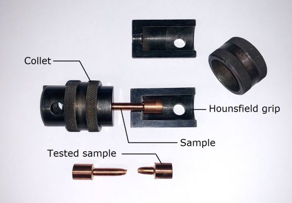
Photo 1: Static image showing a typical tensile specimen and set of grips

Measurement of Load and Displacement

All testing systems have some sort of “loading train”, of which the sample forms a part.  This “train” can be relatively complex  -  for example, it might involve a rotating worm drive (screw thread) somewhere, with the force transmitted to a cross-head and thence via a gripping system to the sample and then to a base-plate of some sort.  It does, of course, need to be arranged that, apart from the sample, all of the components loaded in this way experience only elastic deformation.  The same force (load) is being transmitted along the complete length of the loading train.  Measurement of this load is thus fairly straightforward.  For example, a load cell can be located anywhere in the train, possibly just above the gripping system.  In some simple systems, such as hardness testers or creep rigs, a fixed load may be generated by a dead weight.

Measurement of the displacement (in the gauge length) is more of a challenge.  Sometimes, a measuring device is built into the set-up  -  for example, it could measure the amount of rotation of a worm drive.  In such cases, however, measured displacements include a contribution (elastic) from various elements of the loading train, and this could be quite significant.  It may therefore be important to apply a compliance calibration.  This involves subtracting from the measured displacement the contribution due to the compliance (inverse of stiffness) of the loading train.  This can be measured using a sample of known stiffness (ensuring that it remains elastic).

Displacement Measuring Devices

Several types of device can be used to measure displacement, including Linear Variable Displacement Transducers (LVDTs), eddy current gauges and scanning laser extensometers.  These have resolutions of the order of 1 µm.  More specialised (and accurate) devices include parallel plate capacitors and interferometric optical set-ups, although they often have more limited measurement ranges.

Alternatively, displacement can be measured directly on the gauge length, eliminating concerns about the system compliance. Devices of this type include clip-gauges (knife edges pushing lightly into the sample) and strain gauges (stuck on the sample with adhesive). The latter have good accuracy (±0.1% of the reading), but are limited in range (~1-2% strain). They are useful for measurement of the sample stiffness (Young's modulus), but not for plastic deformation. A versatile technique, useful for mapping strains over a surface, is Digital Image Correlation (DIC), in which the motion of features ("speckles") in optical images is followed automatically during deformation, with displacement resolutions typically of the order of a few μm.

In the video below, which also shows the development of the stress-strain curve, clip gauges are being used to measure the displacement, and hence the strain. It can be seen that, when the strain reaches a certain level (~25% in this case), the specimen starts to"neck". This is apparent in the video and it can also be seen that the onset of necking coincides, at least approximately, with a plateau (peak) in the nominal stress – nominal strain curve. This important phenomenon is examined in more detail on the next page.

 

Video 1: Tensile testing of annealed Cu sample (video and evolving nominal stress-strain plot)

Tensile Testing - Necking and Failure

With a brittle material, tensile testing may give an approximately linear stress-strain plot, followed by fracture (at a stress that may be affected by the presence and size of flaws).  However, most metals do not behave in this way and are likely to experience considerable plastic deformation before they fail.  Initially, this is likely to be uniform throughout the gauge length.

Eventually, of course, it will fail (fracture).  However, in most cases, failure will be preceded by at least some necking.  The formation of a neck is a type of instability, the formation of which is closely tied in with work hardening. It is clear that, once a neck starts to form, the (true) stress there will be higher than elsewhere, possibly leading to more straining there, further reducing the local sectional area and accelerating the effect.

In the complete absence of work hardening, the sample will be very susceptible to this effect and will be prone to necking from an early stage.  (This will be even more likely in a real component under load, where the stress field is likely to be inhomogeneous from the start.)  Work hardening, however, acts to suppress necking, since any local region experiencing higher strain will move up the stress-strain curve and require a higher local stress in order for straining to continue there.  Generally, this is sufficient to ensure uniform straining and suppress early necking.  However, since the work hardening rate often falls off with increasing strain (see earlier page), this balance is likely to shift and may eventually render the sample vulnerable to necking. Furthermore, some materials (with high yield stress and low work hardening rate) may indeed be susceptible to necking from the very start.

Considère’s Construction

This situation was analysed originally by Armand Considère (1885), in the context of the stability of structures such as bridges.  Instability (onset of necking) is expected to occur when an increase in the (local) strain produces no net increase in the load, F.  This will happen when

\[{\rm{\Delta }}F = 0 \qquad \qquad \qquad (8) \]

This leads to

\[F = \sigma A,\qquad \qquad ∴ {\rm{d}}F = A{\rm{d}}\sigma + \sigma {\rm{d}}A = 0\] \[∴ \frac{{{\rm{d}}\sigma }}{\sigma } = \frac{{ - {\rm{d}}A}}{A} = \frac{{{\rm{d}}L}}{L} = {\rm{d}}\varepsilon \] \[∴ \sigma = \frac{{{\rm{d}}\sigma }}{{{\rm{d}}\varepsilon }} \qquad \qquad \qquad (9) \]

Necking is thus predicted to start when the slope of the true stress / true strain curve falls to a value equal to the true stress at that point.  This construction can be explored using the simulation below, in which the true stress – true strain curve is represented by the L-H equation.

 

Simulation 4: Considère's construction (basic construction)

This condition is commonly expressed in terms of the nominal strain.

\[∴ \frac{{{\rm{d}}\sigma }}{{{\rm{d}}\varepsilon }} = \frac{{{\rm{d}}\sigma }}{{{\rm{d}}{\varepsilon _{\rm{N}}}}}\frac{{{\rm{d}}{\varepsilon _{\rm{N}}}}}{{{\rm{d}}\varepsilon }} = \frac{{{\rm{d}}\sigma }}{{{\rm{d}}{\varepsilon _{\rm{N}}}}}\left( {\frac{{{\rm{d}}L/{L_0}}}{{{\rm{d}}L/L}}} \right) = \frac{{{\rm{d}}\sigma }}{{{\rm{d}}{\varepsilon _{\rm{N}}}}}\left( {\frac{L}{{{L_0}}}} \right) = \frac{{{\rm{d}}\sigma }}{{{\rm{d}}{\varepsilon _{\rm{N}}}}}\left( {1 + {\varepsilon _{\rm{N}}}} \right)\] \[∴ \sigma = \frac{{{\rm{d}}\sigma }}{{{\rm{d}}{\varepsilon _{\rm{N}}}}}\left( {1 + {\varepsilon _{\rm{N}}}} \right)\qquad \qquad \qquad (10) \]

The condition can therefore also be formulated in terms of a plot of true stress against nominal strain.  On such a plot, necking will start where a line from the point \(\varepsilon _{\rm{N}} \) = -1 forms a tangent to the curve.  This construction can be explored using the simulation below.

 

Simulation 5: Considère's construction, based on a true stress-nominal strain plot

If the true stress – true strain relationship does conform in this way to the L-H equation, it follows that the necking criterion (Eqn.(9)) can be expressed as

\[{\sigma _{\rm{Y}}} + {K}{\varepsilon ^n} = n{K}{\varepsilon ^{n - 1}} \qquad \qquad \qquad (11) \]

which can be solved analytically.

Ultimate Tensile Stress (UTS) and Ductility

It may be noted at this point that it is common during tensile testing to identify a “strength”, in the form of an “ultimate tensile stress” (UTS).  This is usually taken to be the peak on the nominal stress v. nominal strain plot, which corresponds to the onset of necking.  It should be understood that this value is not actually the true stress acting at failure.  This is difficult to obtain in a simple way, since, once necking has started, the (changing) sectional area is unknown - although the behaviour can often be captured quite accurately via FEM modelling – see below. Also, the "ductility", often taken to be the nominal strain at failure (usually well beyond the strain at the onset of necking) does not correspond to the true strain in the neck when fracture occurs. UTS and ductility values therefore provide only rather loose indications of the strength and toughness of the material. Nevertheless, they are quite widely quoted.

FEM Simulation of Tensile Tests

It is sometimes stated that the initiation of necking during tensile testing arises from (small) variations in sectional area along the gauge length of the sample. However, in practice, for a particular material, its onset does not depend on whether great care has been taken to avoid any such fluctuations. Furthermore, the introduction of such defects in an FEM model does not, in general, significantly affect the predicted onset. The (modelling) condition that does lead to necking is the assumption that, near the end of the gauge length, the sample is constrained from contracting laterally. In practice, due to the increasing sectional area in that region, and because the material beyond the gauge length will undergo little or no deformation, that condition is often a fairly realistic one.

In fact, for any true stress – true strain relationship, including an experimental one that cannot be expressed as an equation, FEM simulation can be used to predict the onset of necking. The simulation below shows, for two materials (with low and high work hardening rates), how the behaviour can be accurately captured and the stress and strain fields explored at any point during the test.(These two materials will also be used to illustrate some effects concerned with compression and indentation testing.) The L-H law is being used here, with best fit values for the 3 parameters in each case.

 

Simulation 6: Tensile test FEM simulation data, for two materials, together with the corresponding videos and experimental stress-strain curves.

 

Compression Testing - Practical Basics, Friction & Barrelling

Uniaxial testing in compression is in many ways simpler and easier than in tension.  There are no concerns about gripping and no possibility of necking or other localised plasticity.  The sample is usually a simple cylinder or cuboid.  However, there are some potential difficulties.  One of these is the danger of (plastic) buckling, particularly if relatively large strains (>~10%) are to be created.  In order to avoid this, the aspect ratio (height / diameter) must be kept relatively low  -  probably not much more than unity.  Since a very large sectional area might lead to excessive load requirements, this often means that the height (gauge length) of the sample is limited.  This in turn leads to relatively low displacements, placing a premium on measurement accuracy (with the points made about compliance calibration, when referring to tensile loading, applying equally here).

Effect of Friction between Sample and Platen

There are also concerns about the effect of friction. This is potentially important, since one outcome of friction is that the stress and strain fields become non-uniform - see the simulation below, so that the nominal stress-strain curve cannot be converted to a true version via use of the analytical equations (even if the value of the coefficient of friction, μ, is known).

In practice, it is common to apply a lubricant to the contact surfaces of the sample and to assume that any effect of friction will be small.  However, the high contact pressure tends to force lubricant out of the region between platen and sample, so this assumption may not be valid.

Two extreme cases can be identified.  The first, which is commonly assumed, is that there is unhindered sliding at the interface (μ = 0).  The sectional area will remain uniform along the sample length during deformation (no barrelling) and there is no frictional work.  The complementary limiting case is that of no sliding.  This also involves no frictional work, but barrelling occurs from the start of the test.  While the exact shape of the “barrel”, as a function of the applied load, will depend on the aspect ratio, it is clear that significant barrelling will invalidate the test  -  the stress now varies along the length of the sample and the relationship between the true stress-strain curve and the outcome will be a complex one.

FEM Simulation

In practice, there is likely to be at least some frictional sliding (with (μ > 0, so that energy is dissipated), but also some barrelling.  The sliding is likely to occur over only part of the surface, since the interfacial shear stress rises with increasing distance from the loading axis (where it is zero).  The outcomes of this can be explored using the simulation below, which is based on FEM modelling.

 

Simulation 7: FEM simulation of a compression test

Indentation Hardness Measurement

Currently, most mechanical testing aimed at obtaining quantitative plasticity characteristics is carried out by uniaxial loading in tension or, to a lesser extent, in compression.  Tensile testing also provides a measure of the “failure strength” (in the form of an “ultimate tensile stress”) and the ductility.  However, these tests require relatively large (uniform) pieces of material, extensive machining to produce samples (at least for tensile testing), considerable care in the way that they are carried out and sound background knowledge in interpretation of the outcome (load-displacement data).  These represent substantial limitations and challenges.

A completely different approach, circumventing virtually all of these difficulties, is that of indentation.  This can be carried out on relatively small samples of simple shape  -  just a flat surface is required, can provide point-to-point mapping of plasticity characteristics over a surface and can be used for non-destructive field testing of components in situ.  It involves pushing a hard indenter into the surface with a known force and measuring the diameter of the resultant indent.  From this measurement, a “hardness number” is obtained.

The indenter must remain elastic  -  ie must experience no plastic deformation -  and is usually made of diamond or another very hard material.  There are several different types of hardness test, including those of Vickers, Brinell, Knoop and Rockwell.  They were all developed several decades ago and they essentially only differ in the shape (and in some cases the material) of the indenter.  A typical hardness test is that of Vickers, the geometry of which is shown below.  The (diamond) indenter is a right pyramid with a square base and an angle of 136˚ between opposite faces. 

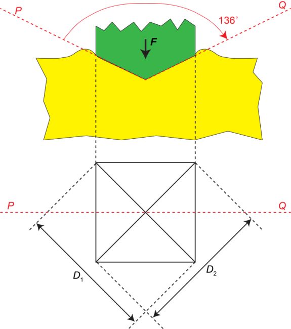
Geometry of the Vickers Hardness Test

The hardness number is the ratio of the applied force, in kgf, to the contact area (NOT the projected area), in mm².  The measured indent diameter, D, taken as the average of D₁ and D₂, IS, however, measured in projection.  The value of H_V is therefore given by

\[{H_{\rm{v}}} = \frac{{2F\sin \left( {\frac{{136}}{2}} \right)}}{{{D^2}}} = 1.854\frac{F}{{{D^2}}} \qquad \qquad \qquad \qquad (12) \]

so a simple calculation allows the hardness number to be obtained from the measured value of D.

There are, of course, certain assumptions incorporated into this analysis.  For example, elastic recovery of the specimen is neglected.  Furthermore, in practice the specimen may exhibit “pile-up” or “sink-in” around the indent, such that the true area of contact differs from that obtained via the simple geometrical picture above.

The stress acting on the contact area (in MPa) is obtained on multiplying the hardness number by 9.81.  However, to say the least, there is no simple relationship between this stress and the stress field generated in the material beneath the indenter.  The latter is complex and also depends in a complex way on the shape of the indenter and the plasticity characteristics of the material.  In fact, even for a given type of hardness, the number obtained tends to vary with the applied load.  This occurs because the load affects the level of plastic strain, which in turn dictates which portions of the stress-strain curve are affecting the outcome.

Nevertheless, it is in practice quite common to use simple expressions so as to obtain a yield stress value from a hardness number.  This is based on the fact that, in the absence of work hardening, and for a given indenter shape, there is an approximately linear relationship between the yield stress (which will be the von Mises stress throughout the volume that has plastically deformed) and the hardness number.  For the Vickers test

\[{\sigma _{\rm{\gamma }}} \approx \frac{{{H_{\rm{v}}}}}{3} \qquad \qquad \qquad \qquad (13) \]

Since very few materials exhibit no work hardening at all, a yield stress obtained in this way is not reliable.  In fact, it is likely to be indicative of a flow stress averaged in some way over the range of plastic strain experienced during the test, which depends on the depth of penetration, the indenter shape and the work hardening characteristics themselves.  It should never be regarded as more than a semi-quantitative indication of the resistance that the material offers to plastic deformation.

Indentation Plastometry

While hardness testing gives only a semi-quantitative indication of the resistance to plastic deformation, the outcome of an indentation operation (ie the size and shape of the residual indent) does depend in a sensitive way on the (true) stress-strain curve of the material, potentially over a large range of plastic strain. Unfortunately, extracting only a single measurement of the indent diameter (while simple experimentally) exploits only a minute proportion of the information incorporated into this residual profile. Measurement of the full profile now forms the basis of a new methodology for obtaining complete (true) stress-strain curves from indentation experiments. This is termed indentation plastometry. Some information about its practical usage is provided in the "Going Further" section.

Before explaining how the procedure works, it should perhaps be emphasized that, even with conventional (uniaxial) tension or compression testing, it is not necessarily straightforward to obtain the correct true stress - true strain relationship. Of course, it is a simple matter to convert nominal stress and nominal strain to true values. However, this is based on the assumption that the sample is deforming uniformly (within the gauge length) throughout the test. In tension, depending on work hardening characteristics, some necking could be taking place - perhaps from a very early stage and quite possibly without it being at all apparent by simply looking at the sample during the test. This will invalidate the standard conversion of nominal stresses and strains to true values. Similarly, in compression testing there is likely to be at least some frictional resistance to interfacial sliding, and hence a degree of barrelling. Again, this invalidates the standard procedure for obtaining the true stress – true strain relationship (although the effect may be relatively small).

For both types of test, as could be inferred from the previous pages, there is a procedure for obtaining the correct stress-strain curve (in the form of the values of the parameters in a constitutive law such as the L-H expression). It involves iterative FEM simulation of the test, evaluating each time a “goodness-of-fit” parameter between the experimental outcome (nominal stress – nominal strain relationship) and that predicted by the model. A search is then made in parameter space, repeatedly simulating the process, until convergence is obtained on the best-fit solution (set of plasticity parameter values). In the case of compression, the value of the coefficient of friction will be part of this parameter set, although it’s likely to have a similar value for a wide range of materials.

In practice, such procedures are rarely carried out for uniaxial testing. Both necking and friction are often simply ignored. In fact, sometimes only nominal stress – nominal strain curves are obtained (although they certainly don’t fully capture the plasticity characteristics and they can’t be used in simulation of more complex multi-axial loading situations). However, there is now a growing awareness that the above methodology can be applied to any loading configuration and, in particular, to indentation (most commonly with a spherical indenter). The experimental outcome can be the load-displacement plot, although it is often more convenient and accurate to use the residual indent profile. Software packages are available for implementing this procedure automatically, with an indication provided about the reliability of the result (fidelity of capturing the actual stress-strain relationship using the constitutive law concerned, with the optimized set of parameter values). The procedure is illustrated below.

FEM Simulation

Iterative FEM simulation of the indentation process is central to the procedure. Starting with some trial (L-H) plasticity parameter values, the simulation is run (to a prescribed load or penetration depth). A comparison is then made between predicted and measured outcomes – either the load-displacement plot or the residual indent profile can be used. This comparison is characterised by the value of a misfit parameter. For the one used in the simulation below, a value below about 10^-3 represents good agreement. A convergence algorithm is used to sequentially select parameter value sets that give improved agreement, until a stable (best fit) combination is obtained. The simulation demonstrates, for the two materials being studied, how this set (and hence the inferred stress-strain curve) is obtained. Outcomes are shown for the initial iteration and then for a few others as the convergence is achieved. It may be noted that a constant value for μ of 0.3 was used in these simulations: experience has shown that this is at least approximately correct for indentation (which is normally unlubricated). If compression testing is carried out with lubrication, then a slightly lower value (~0.15) is likely to be appropriate.

 

Simulation 8: Iterative FEM simulation during indentation plastometry

Comparison between Indentation and Uniaxial Outcomes

There are several ways in which outcomes from these three types of test can be compared. A tensile loading plot of nominal stress against nominal strain is a common one. This allows the UTS (ultimate tensile stress) to be evaluated, since it corresponds (for a metal with at least some ductility) to the peak, where necking is expected to start. Such plots can be obtained by simulation of the tensile test, using sets of L-H parameters obtained by iterative FEM modelling. However, the most convenient way to compare the outcomes is by simply plotting the L-H curves (true stress v. true plastic strain). This is done below. It can be seen that the level of consistency between the 3 methods is good. It is, however, important to understand that it will never be perfect, since an actual (true) stress-strain curve will never conform perfectly to the L-H law (or to any other analytical equation). The most important point here is that, to good accuracy, a plot of this type (and hence a nominal stress v. nominal strain tensile plot) can be extracted solely from indentation data, which can be obtained in a non-destructive way from small samples of simple shape and also from components in use. Such curves are direction-averaged, which should be borne in mind if the material is strongly anisotropic.

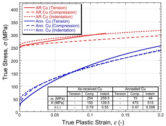
Image 2: Plots, for both materials, of true stress against true (plastic) strain. The tension plots are simply the experimental data, converted to true values, up to the strain level at which necking started. The other two are Ludwik-Hollomon plots, corresponding to the best fit sets of L-H parameter values (shown), obtained via iterative FEM simulation of the compression or indentation tests.

Summary

This TLP has covered the basics of how mechanical testing of metals is carried out, aimed at study of the onset and development of plastic deformation and how it affects the "strength" (failure stress) and ductility. It is based on continuum mechanics - ie there is no detailed consideration of the mechanisms of plasticity or of effects such as anisotropy and inhomogeneity that could arise from microstructural features. The plasticity, and also the consequential necking and fracture that are likely to occur under tensile loading, are characterised by constitutive laws. Two commonly-used expressions are described here. Their usage in FEM modelling is outlined, aimed at obtaining detailed information about the stress and strain fields that are generated during different types of test.

Questions

Quick questions

You should be able to answer these questions without too much difficulty after studying this TLP. If not, then you should go through it again!

1. Which of these statements about deviatoric and hydrostatic stresses and strains is correct, in the context of plastic deformation?

   	a	The deviatoric (von Mises) stress can be positive (tensile) or negative (compressive).
   	b	The equivalent plastic strain (von Mises strain) is always zero.
   	c	The deviatoric (von Mises) stress is a second rank tensor.
   	d	The hydrostatic component of the strain state is always zero.

2. Which of these statements about true and nominal stresses and strains is correct?

   	a	Conversion of nominal stresses and strains to true values, using analytical equations, is only correct if they are uniform throughout the sample.
   	b	It is acceptable to use nominal stress v. nominal strain relationships obtained from uniaxial tests when predicting the behaviour under multi-axial loading.
   	c	The nominal strain is always greater than the true strain.
   	d	The true stress is always greater than the nominal stress.

3. Which of these statements about using constitutive “laws” to describe plastic deformation is correct?

   	a	Constitutive laws are implemented taking account of both the deviatoric and the hydrostatic components of the stress state.
   	b	There is no reason to expect the actual plastic deformation behaviour to conform accurately to any constitutive law.
   	c	Constitutive laws for metal plasticity must predict a continuously decreasing work hardening rate as the strain increases.
   	d	Constitutive laws are based on the assumption that plasticity depends on the peak shear stress generated within the sample.

4. Which of these statements about tensile testing of metals is correct?

   	a	Necking arises in a location where the sample initially has a slightly smaller sectional area.
   	b	Necking arises when the true stress in the location concerned starts to exceed the yield stress.
   	c	Necking of the sample is predicted to start when the gradient of the plot of nominal stress against nominal strain starts to become negative.
   	d	Necking of the sample is predicted to start when the gradient of the plot of true stress against true strain starts to become negative.

5. Which of these statements about compressive testing of metals is correct?

   	a	It is always acceptable to assume that friction between sample and platen has a negligible effect on the outcome, provided that surface is lubricated.
   	b	The complete absence of barreling implies that friction between sample and platen is negligible.
   	c	If there is no sliding between sample and platen, then it is safe to assume that the stress and strain are uniform throughout the test.
   	d	The nominal stress v. nominal strain plot can be converted to a true stress v. true strain plot, using analytical equations, provided there is no interfacial sliding.

6. Which of these statements about hardness testing is correct?

   	a	A hardness number can be used to obtain an accurate value for the yield stress.
   	b	Hardness is defined, for any given applied force, as that force divided by the contact area.
   	c	During hardness testing, the deviatoric stress throughout the plastic zone under the indenter is equal to the yield stress.
   	d	For a given type of hardness test, the value obtained when testing a given sample is independent of the applied force.

7. Which of these statements about indentation plastometry is correct?

   	a	The technique involves repeated numerical simulation of the indentation process, using a constitutive law to represent the true stress v. true strain relationship that applies between the von Mises stress and the equivalent plastic strain.
   	b	The technique involves repeated numerical simulation of the indentation process, using a constitutive law to represent the nominal stress v. nominal strain relationship that applies between the von Mises stress and the equivalent plastic strain.
   	c	The technique involves repeated numerical simulation of the indentation process, using a constitutive law to represent the true stress v. true strain relationship that applies between the hydrostatic stress and the hydrostatic strain.
   	d	The deduced true stress v. true strain relationship will be identical to the curve obtained experimentally during tensile testing, after conversion of nominal stresses and strains to true values, using analytical equations.

Going further

Perhaps unsurprisingly, there are relatively few sources that provide background information regarding something as basic as uniaxial mechanical testing, although there are, of course, plenty of books and websites that cover the fundamentals of stress analysis etc. Among relatively recent books in this area, with an accent on FEM, are the following:

“Practical Stress Analysis with Finite Elements”, Bryan J. MacDonald, Glasnevin publishing (2007), ISBN:978-0-9555781-0-6.
“Structural and Stress Analysis: Theories, Tutorials and Examples”, Jianqiao Ye, Taylor & Francis (2008), ISBN:0-203-02900-3.

Regarding Indentation Plastometry, which is a very recent development, there are as yet no published books and indeed the software necessary to implement the technology is not yet widely available in user-friendly, commercially mature form. However, there are websites that describe the methodology, where such access is likely to become available in due course. Notable among these is https://www.plastometrex.com/..

Academic consultant: Bill Clyne, Jimmy Campbell (University of Cambridge)
Content development: Grey Chen
Photography and video:
Web development: Lianne Sallows and David Brook

DoITPoMS is funded by the UK Centre for Materials Education and the Department , University of Cambridge.