Stress Analysis and Mohr's Circle (all content)

Note: DoITPoMS Teaching and Learning Packages are intended to be used interactively at a computer! This print-friendly version of the TLP is provided for convenience, but does not display all the content of the TLP. For example, any video clips and answers to questions are missing. The formatting (page breaks, etc) of the printed version is unpredictable and highly dependent on your browser.

Main pages

Aims
Before you start
Introduction
Single crystal vs polycrystalline
Representing stress as a tensor
Finding the principal stress tensor
The strain tensor
Yield criteria for metals
Yield criteria for non-metals
Summary
Questions
Going further

Additional pages

Derivation of yield ellipse aspect ratio
Example Problem 1
Example Problem 2

Aims

On completion of this TLP you should:

Recognise the stress and strain tensors and the components into which they can be separated.
Know how to diagonalise a stress tensor for plane stress, and recognise what a principal stress tensor is and why principal stress tensors are useful.
Understand what a yield criterion is and how it can be used.
Have an appreciation of different yield criteria and the materials for which they are appropriate.

Before you start

You should understand the concept of slip and the different ways in which materials (and in particular metals) undergo slip. The Slip in Single Crystals teaching and learning package covers the fundamentals.

In polycrystalline materials, the distribution of grain orientations and the constraint to deformation offered by neighbouring grains gives rise to a simplified overall stress-strain curve in comparison to the curve from a single crystal sample. Crystal structure is also important in polycrystalline samples - the von Mises criterion states that a minimum of five independent slip systems must exist for general yielding.

Introduction

Metal forming involves a permanent change in the shape of a material as a result of the application of an applied stress. The work done in deforming the sample is not recoverable. This plastic deformation involves a change in shape without a change in volume and without melting.

It is desirable to know the stress level at which plastic deformation begins i.e., the onset of yielding. In uniaxial loading, this is the point where the straight, elastic portion of the line first begins to curve. This point is the yield stress. The animation below shows a typical stress-strain curve for a polycrystalline sample, obtained from uniaxial tensile test.

Single crystal vs polycrystalline

The theory of slip in single crystals is well established. When an item is made from metal, however, a single crystal is not generally used. A piece of metal used to make a bicycle or a handrail is made of many small crystals or grains. This affects the behaviour of the metal in many ways:

The grains are not aligned: for example, the [001] axis of one grain might be pointing in a different direction to the [001] axis of its neighbour. This means that different grains slip by different strains when a stress is applied to the whole material, and offer different amounts of resistance to the force. These all contribute to the way that the whole block deforms under stress.

The grain boundaries formed where the grains meet have distinct properties from the rest of the material. When the two crystals either side of a grain boundary have different orientations, defects such as dislocations cannot pass simply through the boundary. Effects like these also have an affect on the response of a metal to stresses.

For these reasons, it is almost impossible to predict in detail from atomic scale theory how a block of metal will deform plastically when a suitable force is applied to it. We must instead find out what happens from experimental observations and then develop a macroscopic engineering model to describe and predict the behaviour of the polycrystalline sample.

Representing stress as a tensor

To understand this page, you first need to understand tensors! Good sources are the books by J.F. Nye [1], G.E. Dieter [2], and D.R. Lovett [3] referred to in the section Going Further in this TLP. Many undergraduate university courses in physical science or engineering have a series of lectures on tensors, such as the course at Cambridge University Department of Materials Science and Metallurgy, the handout for which can be found here.

The stress tensor is a field tensor – it depends on factors external to the material. In order for a stress not to move the material, the stress tensor must be symmetric: σij = σji – it has mirror symmetry about the diagonal.

The general form is thus:

$$\left( {\matrix{ {{\sigma _{11}}} & {{\sigma _{12}}} & {{\sigma _{31}}} \cr {{\sigma _{12}}} & {{\sigma _{22}}} & {{\sigma _{23}}} \cr {{\sigma _{31}}} & {{\sigma _{23}}} & {{\sigma _{33}}} \cr } } \right)$$ or, in an alternative notation, $$\left( {\matrix{ {{\sigma _{xx}}} & {{\tau _{xy}}} & {{\tau _{zx}}} \cr {{\tau _{xy}}} & {{\sigma _{yy}}} & {{\tau _{yz}}} \cr {{\tau _{zx}}} & {{\tau _{yz}}} & {{\sigma _{zz}}} \cr } } \right)$$

The general stress tensor has six independent components and could require us to do a lot of calculations. To make things easier it can be rotated into the principal stress tensor by a suitable change of axes.

Principal stresses

The magnitudes of the components of the stress tensor depend on how we have defined the orthogonal x1, x2 and x3 axes.

For every stress state, we can rotate the axes, so that the only non-zero components of the stress tensor are the ones along the diagonal:

$$\left( {\matrix{ {{\sigma _1}} & 0 & 0 \cr 0 & {{\sigma _2}} & 0 \cr 0 & 0 & {{\sigma _3}} \cr } } \right)$$

that is, there are no shear stress components, only normal stress components.

This is an example of a principal stress tensor of all the tensors we could use to express the stress state that exists. The elements σ1, σ2, σ3 are the principal stresses. The positions of the axes now are the principal axes. While it may be that σ1 > σ2 > σ3, it only matters that the x1, x2 and x3 axes define the directions of the principal stresses.

The largest principal stress is bigger than any of the components found from any other orientation of the axes. Therefore, if we need to find the largest stress component that the body is under, we simply need to diagonalise the stress tensor.

Remember – we have not changed the stress state, and we have not moved or changed the material – we have simply rotated the axes we are using and are looking at the stress state seen with respect to these new axes.

Hydrostatic and deviatoric components

The stress tensor can be separated into two components. One component is a hydrostatic or dilatational stress that acts to change the volume of the material only; the other is the deviatoric stress that acts to change the shape only.

$$\left( {\matrix{ {{\sigma _{11}}} & {{\sigma _{12}}} & {{\sigma _{31}}} \cr {{\sigma _{12}}} & {{\sigma _{22}}} & {{\sigma _{23}}} \cr {{\sigma _{31}}} & {{\sigma _{23}}} & {{\sigma _{33}}} \cr } } \right) = \left( {\matrix{ {{\sigma _H}} & 0 & 0 \cr 0 & {{\sigma _H}} & 0 \cr 0 & 0 & {{\sigma _H}} \cr } } \right) + \left( {\matrix{ {{\sigma _{11}} - {\sigma _H}} & {{\sigma _{12}}} & {{\sigma _{31}}} \cr {{\sigma _{12}}} & {{\sigma _{22}} - {\sigma _H}} & {{\sigma _{23}}} \cr {{\sigma _{31}}} & {{\sigma _{23}}} & {{\sigma _{33}} - {\sigma _H}} \cr } } \right)$$

where the hydrostatic stress is given by ${\sigma _H}$ = ${1 \over 3}$$\left( {{\sigma _1} + {\sigma _2} + {\sigma _3}} \right)$.

In crystalline metals plastic deformation occurs by slip, a volume-conserving process that changes the shape of a material through the action of shear stresses. On this basis, it might therefore be expected that the yield stress of a crystalline metal does not depend on the magnitude of the hydrostatic stress; this is in fact exactly what is observed experimentally.

In amorphous metals, a very slight dependence of the yield stress on the hydrostatic stress is found experimentally.

Finding the principal stress tensor

Rotating the axes:

The principal stresses are the eigenvalues of the stress tensor. These can be found from the determinant equation:

$$\left| {\begin{array}{*{20}{c}} {{\sigma _{11}} - \xi }&{{\sigma _{12}}}&{{\sigma _{13}}}\\ {{\sigma _{21}}}&{{\sigma _{22}} - \xi }&{{\sigma _{23}}}\\ {{\sigma _{31}}}&{{\sigma _{32}}}&{{\sigma _{33}} - \xi } \end{array}} \right| = 0$$

This determinant is expanded out to produce a cubic equation from which the three possible values of $\xi $ can be found; these values are the principal stresses. This is discussed in the book by J.F. Nye [1].

If the stress tensor already has a principal stress along one axis, such as σ33, diagonalising is much simpler:

$$\left| {\begin{array}{*{20}{c}} {{\sigma _{11}} - \xi }&{{\sigma _{12}}}&0\\ {{\sigma _{21}}}&{{\sigma _{22}} - \xi }&0\\ 0&0&{{\sigma _{33}} - \xi } \end{array}} \right| = 0$$

When we expand this out, we find that:

\[({\sigma _{33}} - \xi )\left[ {({\sigma _{11}} - \xi )({\sigma _{22}} - \xi ) - \sigma _{12}^2} \right] = 0\]

One of the principal stresses must be σ33, and the other two are easy to find by solving the quadratic equation inside the square brackets for $\xi $. Alternatively, when there are only two principal stresses to find, such as in this example, we can use Mohr’s circle.

Mohr’s circle method:

Mohr’s circle in this situation represents a stress state, on two axes – normal (σ) and shear (τ). A Mohr's circle drawn according to the convention in Gere and Timoshenko [4] in shown below.

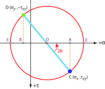
The normal stresses σx and σy are first plotted on the horizontal σ axis at A and B. Positions C and D are then generated using the magnitude of the shear stress τxy, with the convention for the choice of these positions shown. Different orientations of the axes, and the different stress tensors produced by them, are represented by the different diameters it is possible to take of the circle.

The principal stress state is the state which has no shear components. This corresponds to the diameter of the Mohr’s circle that has no component along the shear axis – it is the diameter that runs along the normal stress axis. The principal stresses are thus the two points where the circle crosses the normal stress axis, E and F:

$$\left( {\begin{array}{*{20}{c}} E&0&0\\ 0&F&0\\ 0&0&{{\sigma _3}} \end{array}} \right)$$

The angle 2θ shown on the Mohr's circle in an anti-clockwise sense is twice the angle θ required to rotate the set of axes in an anti-clockwise sense from the old set of axes to the principal axes with respect to which the principal stresses are defined.

The Mohr’s circle below is for an element under a stress state of σ11= 80 MPa, σ22 = – 60 MPa, σ12 = 50 MPa and σ3 = 100 MPa. Using the slider, change its inclination angle and compare it to the tensor representing the stress state.

Given below is an interactive tool to plot a Mohr's circle according to user's specified stress states.

The strain tensor

When stress is applied to the material, strain is produced. Strain is also a symmetric second-rank tensor. Stress and strain are related by:

σij = Cijklεkl

The strain tensor, εkl, is second-rank just like the stress tensor. The tensor that relates them, Cijkl, is called the stiffness tensor and is fourth-rank.

Alternatively:

εij= Sijklσkl

Sijkl is called the compliance tensor and is also fourth-rank.

The strain tensor is a field tensor – it depends on external factors. The compliance tensor is a matter tensor – it is a property of the material and does not change with external factors.

Expressing the strain in a slip process in terms of displacement

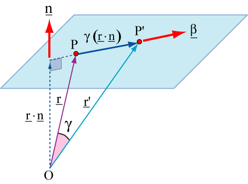
This diagram shows a plane on which slip occurs. A general point P is moved to position P' by the slip. The vectors from the origin to P and P' are r and r' respectively. Also shown is the unit vector n > normal to the plane, and β perpendicular to the plane from O. The length of the perpendicular from O to the plane is simply r·n. Unit vector n has components of n₁, n₂, n₃, and r has components of x₁, x₂, x₃.

Suppose the distance moved in the direction of slip is $\gamma \left( {\underset{\raise0.3em\hbox{$\smash{\scriptscriptstyle-}$}}{r} \cdot \underset{\raise0.3em\hbox{$\smash{\scriptscriptstyle-}$}}{n} } \right)$. The displacement vector that represents slip is then given by:

$$\underset{\raise0.3em\hbox{$\smash{\scriptscriptstyle-}$}}{r} ' - \underset{\raise0.3em\hbox{$\smash{\scriptscriptstyle-}$}}{r} = \gamma \left( {\underset{\raise0.3em\hbox{$\smash{\scriptscriptstyle-}$}}{r} \cdot \underset{\raise0.3em\hbox{$\smash{\scriptscriptstyle-}$}}{n} } \right)\underset{\raise0.3em\hbox{$\smash{\scriptscriptstyle-}$}}{\beta } $$

where β is a unit vector in the direction of slip and has components of b₁, b₂ and b₃.

If the strain angle is small, the components of the deformation tensor eij can be obtained by differentiating the displacements, so that

$${e_{ij}} = {{\partial {u_i}} \over {\partial {x_j}}} = {\partial \over {\partial {x_j}}}\gamma \left( {{\underset{\raise0.3em\hbox{$\smash{\scriptscriptstyle-}$}}{r} \cdot \underset{\raise0.3em\hbox{$\smash{\scriptscriptstyle-}$}}{n} } } \right){\beta _i}$$

Hence, for example,

$${e_{11}} = {{\partial {u_1}} \over {\partial {x_1}}} = {\partial \over {\partial {x_1}}}\gamma \left( {{\underset{\raise0.3em\hbox{$\smash{\scriptscriptstyle-}$}}{r} \cdot \underset{\raise0.3em\hbox{$\smash{\scriptscriptstyle-}$}}{n} } } \right){\beta _1} = \gamma {\beta _1}{\partial \over {\partial {x_1}}}\left( {{x_1}{n_1} + {x_2}{n_2} + {x_3}{n_3}} \right) = \gamma {n_1}{\beta _1}$$

More generally,

$${e_{ij}} = {{\partial {u_i}} \over {\partial {x_j}}} = \gamma {n_j}{\beta _i}$$

We can then write the tensor like this:

$${e_{ij}} = \gamma \left( {\matrix{ {{n_1}{\beta _1}} & {{n_2}{\beta _1}} & {{n_3}{\beta _1}} \cr {{n_1}{\beta _2}} & {{n_2}{\beta _2}} & {{n_3}{\beta _2}} \cr {{n_1}{\beta _3}} & {{n_2}{\beta _3}} & {{n_3}{\beta _3}} \cr } } \right)$$ $${\varepsilon _{ij}} = \gamma \left( {\matrix{ {{n_1}{\beta _1}} & {{1 \over 2}\left( {{n_2}{\beta _1} + {n_1}{\beta _2}} \right)} & {{1 \over 2}\left( {{n_3}{\beta _1} + {n_1}{\beta _3}} \right)} \cr {{1 \over 2}\left( {{n_1}{\beta _2} + {n_2}{\beta _1}} \right)} & {{n_2}{\beta _2}} & {{1 \over 2}\left( {{n_3}{\beta _2} + {n_2}{\beta _3}} \right)} \cr {{1 \over 2}\left( {{n_1}{\beta _3} + {n_3}{\beta _1}} \right)} & {{1 \over 2}\left( {{n_2}{\beta _3} + {n_3}{\beta _2}} \right)} & {{n_3}{\beta _3}} \cr } } \right)$$

Separation of the strain tensor

Notice that the tensor derived from the diagram is e_ij while the strain tensor related to the stress tensor by the stiffness and compliance tensors is εij. This is not a mistake!

The tensor eij derived from the diagram describes the specimen moving relative to the origin. This includes a change in dimension of the specimen, the strain. It also may include a rotation of the specimen. In terms of the properties of the material, the rotation is not of interest, so we must separate it out to be left with the strain alone.

eij = εij + ωij

where εij is the strain tensor and ωij is the rotation tensor.

$${\omega _{ij}} = \gamma \left( {\matrix{ 0 & {{1 \over 2}\left( {{n_2}{\beta _1} - {n_1}{\beta _2}} \right)} & {{1 \over 2}\left( {{n_3}{\beta _1} - {n_1}{\beta _3}} \right)} \cr {{1 \over 2}\left( {{n_1}{\beta _2} - {n_2}{\beta _1}} \right)} & 0 & {{1 \over 2}\left( {{n_3}{\beta _2} - {n_2}{\beta _3}} \right)} \cr {{1 \over 2}\left( {{n_1}{\beta _3} - {n_3}{\beta _1}} \right)} & {{1 \over 2}\left( {{n_2}{\beta _3} - {n_3}{\beta _2}} \right)} & 0 \cr } } \right)$$

A strain tensor must be symmetrical. A rotation tensor must be antisymmetric. The rotation tensor must also have no normal components. The strain tensor εij is the one used in calculations.

Volumetric strain

The sum of the diagonal elements of the strain tensor is the volumetric strain or dilatation:

$${{\Delta V} \over V} = {\varepsilon _{11}} + {\varepsilon _{22}} + {\varepsilon _{33}} = \Delta $$

The volumetric strain for metals during plastic deformation is zero. Hence, during plastic deformation there are five independent components, rather than six, of the general strain tensor, describing an incremental change of shape.

Yield criteria for metals

A yield criterion is a hypothesis defining the limit of elasticity in a material and the onset of plastic deformation under any possible combination of stresses.

There are several possible yield criteria. We will introduce two types here relevant to the description of yield in metals.

To help understanding of combinations of stresses, it is useful to introduce the idea of principal stress space. The orthogonal principal stress axes are not necessarily related to orthogonal crystal axes.

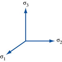
Using this construction, any stress can be plotted as a point in 3D stress space.

For example, the uniaxial stress $\left( {\begin{array}{*{20}{c}} \sigma &0&0\\ 0&0&0\\ 0&0&0 \end{array}} \right)$ where σ1 = σ; σ2 = σ3= 0, plots as a point on the σ1axis.

A purely hydrostatic stress σ1 = σ2 = σ3=σH will lie along the vector [111] in principal stress space. For any point on this line, there can be no yielding, since in metals, it is found experimentally that hydrostatic stress does not induce plastic deformation (see hydrostatic and deviatoric components).

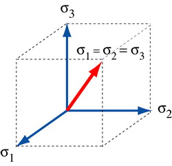The 'hydrostatic line'

We know from uniaxial tension experiments, that if σ1 = Y, σ2 = σ3 = 0 where Y is a uniaxial stress, then yielding will occur.

Therefore, there must be a surface, which surrounds the hydrostatic line and passes through (Y, 0, 0) that defines the boundary between elastic and plastic behaviour. This surface will define a yield criterion. Such a surface has also to pass through the points (0, Y, 0), (0, 0, Y), (–Y, 0, 0) (0, –Y, 0) and (0, 0, –Y).

The plane defined by the three points (Y, 0, 0), (0, Y, 0) and (0, 0, Y) is parallel to the plane defined by the three points (–Y, 0, 0) (0, –Y, 0) and (0, 0, –Y).

The simplest shape for a yield criterion satisfying these requirements is a cylinder of appropriate radius with an axis along the hydrostatic line. This can be described by an equation of the form:

\[{\left( {{\sigma _1} - {\sigma _2}} \right)^2} + {\left( {{\sigma _2} - {\sigma _3}} \right)^2} + {\left( {{\sigma _3} - {\sigma _1}} \right)^2} = {\rm{constant}}\]

From above, if, σ₁ = Y, σ₂ = σ₃= 0, then the constant is given by 2Y². This is the von Mises Yield Criterion.

We can also define a yield stress in terms of a pure shear, k. A pure shear stress can be represented in a Mohr’s Circle, as follows:

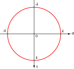
Referred to principal stress space, we have σ₁ = k, σ₂ = –k, σ₃= 0.

The von Mises criterion can therefore be expressed as:

\[2{Y^2} = 6{k^2}{\rm{ }} \Rightarrow {\rm{ }}Y = k\sqrt 3 \]

A mathematically simpler criterion which satisfies the requirements for the yield surface having to pass through (Y, 0, 0), (0, Y, 0) and (0, 0, Y) is the Tresca Criterion.

If we suppose σ1 > σ2> σ3, then the largest difference between principal stresses is given by (σ₁ – σ₃).

If yielding occurs when σ1 = Y, σ2 = σ3= 0, then (σ1 – σ3) = Y.

For yield in pure shear at some shear stress k, when referred to the principal stress state we could have

\[{\sigma _1} = k,{\rm{ }}{\sigma _2} = 0,{\rm{ }}{\sigma _3} = - k{\rm{ }} \Rightarrow {\rm{ }}Y = 2k\]

The Tresca criterion is (σ1 – σ3) = Y = 2k.

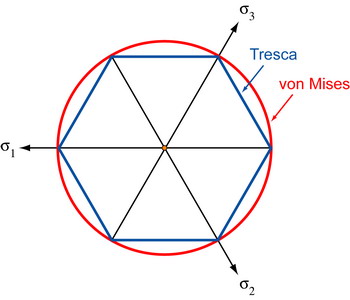
Viewed down the hydrostatic line, the two criteria appear as:

For plane stress, let the principal stresses be σ1 and σ2, with σ3= 0.

The yield surfaces for the Tresca yield criterion and the von Mises yield criterion in plane stress are shown below:

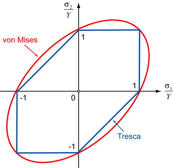
The Tresca yield surface is an irregular hexagon and the von Mises yield surface is an ellipse. The ratio of the length of the major and minor axes of this ellipse is $\sqrt 3 {\rm{ :1}}$. Click here for a derivation of this result.

Experiments suggest that the von Mises yield criterion is the one which provides better agreement with observed behaviour than the Tresca yield criterion. However, the Tresca yield criterion is still used because of its mathematical simplicity.

Example Problem 1: Yield criteria for metals

Yield criteria for non-metals

When ceramics deform plastically (usually only at temperatures very close to their melting point, if at all), they often obey the von Mises or Tresca criterion.

However, other materials such as polymers and geological materials (rocks and soils) display yield criteria that are not independent of hydrostatic pressure.

Empirically, it is found that as a hydrostatic pressure is increased, the yield stress increases, and so we do not expect a yield criterion based solely on the deviatoric component of stress to be valid.

The first attempt to produce a yield criterion incorporating the effect or pressure was derived by Coulomb.

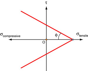
The Coulomb criterion

Failure occurs when the shear stress, τ, on any plane reaches a critical value, τ_c, which varies linearly with the stress normal to that plane.

\[{\tau _c} = {\tau ^*} - {\sigma _n}\tan \phi \]

where is the positive normal stress on the plane of failure (so that on this convention, a compressive stress or pressure is a negative quantity), is a material parameter and is the angle of shearing resistance. (Note: is not a ‘coefficient of friction’ although often referred to as such).

Failure locus for soil

For soils, tanφ ≈ 0.5 - 0.6 typically. So as a soil is compressed, τ_c increases.

If the principal components of stress are σ1, σ2, σ3 for a particular stress state at some point within a soil mass, we can draw three Mohr’s circles with diameters specified by σ1 > σ3 ; σ2 > σ3 ; σ1> σ2. For failure, we require only one of these to touch the failure locus, e.g.

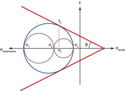
Here, failure is determined by $\left| {{\sigma _1} - {\sigma _3}} \right|$, not by σ2. This is therefore a variant or modification of the Tresca criterion.

Example Problem 2: Yield criteria for non-metals

A better model for polymers is to assume that the shear stress k at which failure occurs is a function of hydrostatic stress or pressure, e.g.

$$k = {k_0} + \mu P$$

where $P = - $$\frac{1}{3}$$\left( {{\sigma _1} + {\sigma _2} + {\sigma _3}} \right) = - {\sigma _H}$ = hydrostatic pressure and k0 is the value of shear yield stress at zero hydrostatic pressure.

If we do this, we obtain pressure-modified criteria, which work well for polymers. For example, the pressure-modified von Mises criterion has a circular sectional cone with its axis along σ1 = σ2 = σ3:

$${\left( {{\sigma _1} - {\sigma _2}} \right)^2} + {\left( {{\sigma _2} - {\sigma _3}} \right)^2} + {\left( {{\sigma _3} - {\sigma _1}} \right)^2} = 2{Y^2} = 6{k^2} = 6\left( {{k_o} + \mu P} \right)$$

The pressure-modified Tresca criterion has a hexagonal pyramid with axis along σ1 = σ2 = σ3:

$$\left( {{\sigma _1} - {\sigma _3}} \right) = Y = 2k = 2\left( {{k_0} + \mu P} \right)$$

These modified criteria work well for polymers.

Summary

Stress and strain and the relationship between them can be expressed in tensor formalism.

The stress tensor is symmetric and can be separated into hydrostatic and deviatoric components.

The stress state can be expressed by a tensor that has only diagonal components – the principal stress tensor. This is achieved by rotating the axes of the stress tensor, so that the axes are parallel to the forces on the body.

The measured strain tensor can be separated into a symmetric real strain tensor and an antisymmetric rotation tensor. The real strain tensor can then be separated into dilatational (volume expansion) and deviatoric (shape change) components.

We can define combinations of the three principal stress components that will cause yield – yield criteria. Different criteria are best used for different materials. The best one for metals is the von Mises yield criterion:

$${({\sigma _1} - {\sigma _2})^2} + {({\sigma _2} - {\sigma _3})^2} + {({\sigma _3} - {\sigma _1})^2} = 6{k^2} = 2{Y^2}$$

A mathematically simpler approximation to the von Mises yield criterion is the Tresca yield criterion:

$$\frac{{\left( {{\sigma _1} - {\sigma _3}} \right)}}{2} = k = \frac{Y}{2}$$

If a yield criterion is plotted in 3D stress space, we have a yield surface.

Questions

Quick questions
You should be able to answer these questions without too much difficulty after studying this TLP. If not, then you should go through it again!

Use the interactive Mohr's circle below to help you with this question. Which of these stress states is not the same as the others?

a

b

c

d

What kind of movement are these tensors - rotation, strain or both? Click on each and check the answer.

a

b

c

d

The yield stress of an aluminium alloy in uniaxial tension is 320 MPa. The same alloy also yields under the combined stress state:
Is the behaviour of this alloy better described by the von Mises or the Tresca yield criterion?

Going further

Books

[1] J.F. Nye, Physical Properties of Crystals, Oxford, 1985.

[2] G.E. Dieter, Mechanical Metallurgy, 3^rd Edition, McGraw-Hill, 1990.

[3] D.R. Lovett, Tensor Properties of Crystals, 2^nd Edition, Adam Hilger, 1999.

[4] B.J. Goodno and J,M, Gere, Mechanics of Materials. 9^th Edition, Cengage, 2018.

[5] A. Kelly and K.M. Knowles, Crystallography and Crystal Defects, 3^rd Edition, Wiley, 2020.

Derivation of yield ellipse aspect ratio

For plane stress, let the principal stresses be ${\sigma _1}$ and ${\sigma _2}$, with ${\sigma _3} = 0$.

The yield surfaces for the Tresca yield criterion and the von Mises yield criterion are shown below.

The Tresca yield surface is an irregular hexagon and the von Mises yield surface is an ellipse. The ratio of the length of the major and minor axes of this ellipse is $\sqrt 3 {\rm{ :1}}$.

In the quadrant where ${\sigma _1} > 0$ and ${\sigma _2} > 0$, the Tresca yield surface is a square.

To see this, first suppose ${\sigma _1} > {\sigma _2}$ for example. Since ${\sigma _3} < {\sigma _2}$, yield occurs on the Tresca criterion when

\[{\sigma _1} - {\sigma _3} = Y\]

i.e., for ${\sigma _1} = Y$ because ${\sigma _3} = 0$. When ${\sigma _1} = {\sigma _2}$, yield occurs at ${\sigma _1} = {\sigma _2} = Y$. Similarly, for ${\sigma _1} < {\sigma _2}$ in this quadrant, yield occurs when ${\sigma _2} = Y$.

The shape of the Tresca yield surface in the quadrant where ${\sigma _1} > 0$ and ${\sigma _2} < 0$ is a straight line because the third principal stress ${\sigma _3}$ will be the intermediate principal stress. Hence in this quadrant the yield criterion becomes

\[\left| {{\sigma _1} - {\sigma _2}} \right| = Y\]

whence the straight line linking (-1,0) to (0,1) in the diagram. The shape of the Tresca yield surface in the remaining two quadrants follows similarly.

For plane stress the von Mises yield criterion becomes

$${\left( {{\sigma _1} - {\sigma _2}} \right)^2} + {\sigma _2}^2 + {\sigma _1}^2 = 2{Y^2}$$

which for Y = 1 becomes

$$2{\sigma _1}^2 + 2{\sigma _2}^2 - 2{\sigma _1}{\sigma _2} = 2$$

i.e.,

$${\sigma _1}^2 + {\sigma _2}^2 - {\sigma _1}{\sigma _2} = 1$$

Thus the yield surface for plane stress passes through (1,0), (1,1) (0,1) (-1,0) (-1,-1), and (0,-1). It also passes through the points

$$\left( { - \frac{1}{{\sqrt 3 }},\frac{1}{{\sqrt 3 }}} \right){\rm{ and }}\left( {\frac{1}{{\sqrt 3 }}, - \frac{1}{{\sqrt 3 }}} \right)$$

as can be seen by direct substitution in the yield condition for ${\sigma _1} = -{\sigma _2}$.

The directions

$$\left[ {{\rm{1,1}}} \right]{\rm{ and }}\left[ {\frac{1}{{\sqrt 3 }}, - \frac{1}{{\sqrt 3 }}} \right]$$

are orthogonal and their magnitudes define the length of the major and minor axes of this ellipse.

Hence, the ratio of the length of the major and minor axes of this ellipse is $\sqrt 3 {\rm{ :1}}$.

Example Problem 1

Example Problem 2

Academic consultant: Kevin Knowles (University of Cambridge)
Content development: Andrew Bennett, Joanne Sharp
Web development: Jin Chong Tan and Lianne Sallows

This DoITPoMS TLP was funded by the UK Centre for Materials Education and the Department of Materials Science and Metallurgy, University of Cambridge.