Finite Element Method (all content)

Note: DoITPoMS Teaching and Learning Packages are intended to be used interactively at a computer! This print-friendly version of the TLP is provided for convenience, but does not display all the content of the TLP. For example, any video clips and answers to questions are missing. The formatting (page breaks, etc) of the printed version is unpredictable and highly dependent on your browser.

Contents

Aims

On completion of this TLP you should:

• Understand the basics of the finite element method
• Be familiar with the concepts of nodes, elements and discretisation
• Understand the direct stiffness method
• Be able to construct an element stiffness matrix and a global stiffness matrix for 1-dimensional elements
• Appreciate the importance of boundary conditions
• Understand shape (interpolation) functions for 1-dimensional elements
• Understand the difference between linear and non-linear static finite element problems
• Be familiar with some common reasons for non-convergence

Before you start

There are no special prerequisites for this TLP, but it would be useful to be familiar with stress and strain, beam bending mechanics and matrices (see Tensors in Materials Science).

Introduction

Overview

The Finite Element Method (FEM) is a mathematical (numerical) technique for finding approximate solutions to partial differential equations. It is a technique which is very well suited to the study and analysis of complex physical phenomena, particularly those exhibiting non-linearity in geometry and/or material behaviour (which is often the case for most “real-world” situations). It is used frequently to tackle problems that are not readily amenable to analytical treatments. Such problems can be structural, thermal, electrical, magnetic, acoustic etc., either in isolation or when coupled. Coupled examples include (but are not limited to) thermomechanical – where constrained differential thermal expansion generates thermal-stresses, thermoelectric – where heat is generated in a material due to its resistance to current flow, and conjugate heat transfer – where moving fluids can remove heat from hot objects over which they pass. When the Finite Element Method is used to solve problems of this type it is often referred to as Finite Element Analysis (FEA).

Premise

The premise is very simple; continuous domains (geometries) are decomposed into discrete, connected regions (or Finite Elements). An assembly of element-level equations is subsequently solved, while conditions of kinematic compatibility are enforced, in order to establish the response of the complete domain to a particular set of boundary conditions. The premise is described to some degree in the figure below, which also lists the governing equations (in differential form) for a range of common physical phenomena (in 1-D).

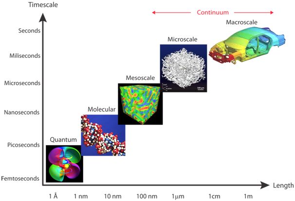
Time and Lengthscales

Typical time and lengthscales for application of the finite element method are shown in the following figure.

Example Videos:

The videos below have been produced from finite element analyses and include:

FEM of plate perforation

Punch

Nodes, elements, degrees of freedom and boundary conditions

“Nodes”, “Elements”, “Degrees of Freedom” and “Boundary Conditions” are important concepts in Finite Element Analysis.

When a domain (a geometric region) is meshed, it is decomposed into a series of discrete (hence finite) ELEMENTS. The meshed geometry of an exhaust manifold is shown in the figure below. It can be seen that the elements in the mesh conform very well to the geometry, and represent therefore a good approximation of the geometry. The manifold in this instance is meshed with a 3-dimensional brick element which contains 20 NODES. Adjacent elements are connected to each other AT the nodes. A node is simply a point in space, defined by its coordinates, at which DEGREES OF FREEDOM are defined. In finite element analysis a degree of freedom can take many forms, but depends on the type of analysis being performed. For instance, in a structural analysis the degrees of freedom are displacements (U_x, U_y and U_z), while in a thermal analysis the degree of freedom is temperature (T). In the exhaust manifold example, there are 4 degrees of freedom at each node – U_x, U_y, U_z and T, since the analysis is a coupled temperature-displacement analysis (due to thermal expansion effects).  These FIELD VARIABLES are calculated at every node from the governing equation. Field variable values between the nodes and within the elements are calculated using interpolation functions, which are sometimes called shape or base functions.

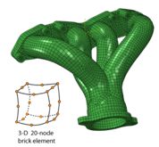
Manifold and node map

There are of course many types of element, covering the complete range of space dimension. The most common are shown in the figure below, along with the position of the nodes, where It can be seen that some of the elements have “midside” nodes – i.e. nodes positioned midway between the corner nodes. The edges of these “higher order” elements can therefore curve – making them suitable for capturing complex geometrical shapes (as in the manifold above). This is possible since these elements permit the solution between the nodes to vary in non-linear ways (see section on shape functions), which is an important feature when field variables change rapidly.

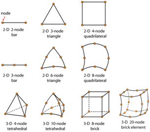
Examples of FEM element types

Boundary Conditions

Boundary conditions are specified values of the field variables (or their derivatives) on the boundaries of the field (the geometry). They fall in to three categories: Dirichlet conditions – where you prescribe the variable for which you are solving; Neumann conditions – where you prescribe a flux, which is the gradient of the dependent variable, and Robin conditions – which is a mixture of the two, where a relation between the variable and its gradient is prescribed. The following table features some examples from various physical fields that show the corresponding physical interpretation.

Physics	Dirichlet	Neumann	Robin
Solid Mechanics	Displacement	Traction (Stress)	Spring
Heat Transfer	Temperature	Heat Flux	Convection
Pressure Acoustics	Acoustic Pressure	Normal Acceleration	Impedance
Electric Currents	Fixed Potential	Fixed Current	Impedance

Direct stiffness method and the global stiffness matrix

Although there are several finite element methods, we analyse the Direct Stiffness Method here, since it is a good starting point for understanding the finite element formulation. We consider first the simplest possible element – a 1-dimensional elastic spring which can accommodate only tensile and compressive forces. For the spring system shown, we accept the following conditions:

• Condition of Compatibility – connected ends (nodes) of adjacent springs have the same displacements
• Condition of Static Equilibrium – the resultant force at each node is zero
• Constitutive Relation – that describes how the material (spring) responds to the applied loads

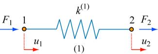
Model spring system

The constitutive relation can be obtained from the governing equation for an elastic bar loaded axially along its length:
\[\frac{d}{{du}}\left( {AE\frac{{\Delta l}}{{{l_0}}}} \right) + k = 0 \;\;\;\;\;(1)\] \[\frac{{\Delta l}}{{{l_0}}} = \varepsilon \;\;\;\;\;(2) \] \[\frac{d}{{du}}\left( {AE\varepsilon } \right) + k = 0 \;\;\;\;\;(3) \] \[\frac{d}{{du}}\left( {A\sigma } \right) + k = 0 \;\;\;\;\;(4) \] \[\frac{{dF}}{{du}} + k = 0 \;\;\;\;\;(5) \] \[\frac{{dF}}{{du}} = - k \;\;\;\;\;(6) \] \[dF = - kdu \;\;\;\;\;(7) \]

The spring stiffness equation relates the nodal displacements to the applied forces via the spring (element) stiffness. The minus sign denotes that the force is a restoring one, but from here on in we use the scalar version of Eqn.7.

Derivation of the Stiffness Matrix for a Single Spring Element

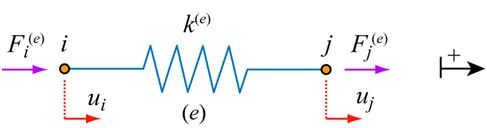
From inspection, we can see that there are two degrees of freedom in this model, u_i and u_j.  We can write the force equilibrium equations:

\[{k^{\left( e \right)}}{u_i} - {k^{\left( e \right)}}{u_j} = F_i^{\left( e \right)} \;\;\;\;\;(8) \] \[ - {k^{\left( e \right)}}{u_i} + {k^{\left( e \right)}}{u_j} = F_j^{\left( e \right)} \;\;\;\;\;(9) \]

In matrix form
\[\left[ {\begin{array}{*{20}{c}}{{k^e}}&{ - {k^e}}\\{ - {k^e}}&{{k^e}}\end{array}} \right]\left\{ {\begin{array}{*{20}{c}}{{u_i}}\\{{u_j}}\end{array}} \right\} = \;\left\{ {\begin{array}{*{20}{c}}{F_i^{\left( e \right)}}\\{F_j^{\left( e \right)}}\end{array}} \right\} \;\;\;\;\;(10) \]

The order of the matrix is [2×2] because there are 2 degrees of freedom. Note also that the matrix is symmetrical. The ‘element’ stiffness relation is:

\[[{K^{(e)}}]\{ {u^{(e)}}\} = \{ {F^{(e)}}\} \;\;\;\;\;(11) \]

Where Κ^(e) is the element stiffness matrix, u^(e) the nodal displacement vector and F^(e) the nodal force vector. (The element stiffness relation is important because it can be used as a building block for more complex systems. An example of this is provided later.)

Derivation of a Global Stiffness Matrix

For a more complex spring system, a ‘global’ stiffness matrix is required – i.e. one that describes the behaviour of the complete system, and not just the individual springs.

 

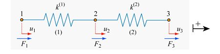
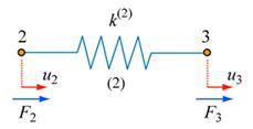
From inspection, we can see that there are two springs (elements) and three degrees of freedom in this model, u₁, u₂ and u₃. As with the single spring model above, we can write the force equilibrium equations:
\[{k^1}{u_1} - {k^1}{u_2} = {F_1} \;\;\;\;\;(12) \] \[ - {k^1}{u_1} + \left( {{k^1} + {k^2}} \right){u_2} - {k^2}{u_3} = {F_2} \;\;\;\;\;(13) \] \[{k^2}{u_3} - {k^2}{u_2} = {F_3 \;\;\;\;\;(14) }\]

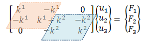
In matrix form \[\left[ {\begin{array}{*{20}{c}} {{k^1}}&{ - {k^1}}&0\\ { - {k^1}}&{{k^1} + {k^2}}&{ - {k^2}}\\ 0&{ - {k^2}}&{{k^2}} \end{array}} \right]\left\{ {\begin{array}{*{20}{c}} {{u_1}}\\ {{u_2}}\\ {{u_3}} \end{array}} \right\} = \;\left\{ {\begin{array}{*{20}{c}} {{F_1}}\\ {{F_2}}\\ {{F_3}} \end{array}} \right\} \;\;\;\;\;(15) \]

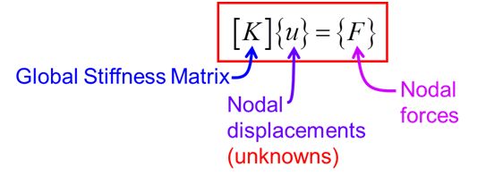
The ‘global’ stiffness relation is written in Eqn.16, which we distinguish from the ‘element’ stiffness relation in Eqn.11. \[\left[ K \right]\left\{ u \right\} = \;\left\{ F \right\} \;\;\;\;\;(16) \]

Note the shared k¹ and k² at k²² because of the compatibility condition at u₂. We return to this important feature later on.

Assembling the Global Stiffness Matrix from the Element Stiffness Matrices

Although it isn’t apparent for the simple two-spring model above, generating the global stiffness matrix (directly) for a complex system of springs is impractical. A more efficient method involves the assembly of the individual element stiffness matrices. For instance, if you take the 2-element spring system shown,

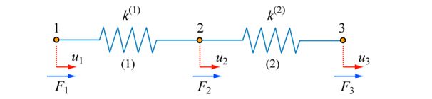
split it into its component parts in the following way

    

and derive the force equilibrium equations \[{k^1}{u_1} - {k^1}{u_2} = {F_1} \;\;\;\;\;(17) \] \[{k^1}{u_2} - {k^1}{u_1} = {k^2}{u_2} - {k^2}{u_3} = {F_2} \;\;\;\;\;(18) \] \[{k^2}{u_3} - {k^2}{u_2} = {F_3} \;\;\;\;\;(19) \] then the individual element stiffness matrices are: \[\left[ {\begin{array}{*{20}{c}} {{k^1}}&{ - {k^1}}\\ { - {k^1}}&{{k^1}} \end{array}} \right]\left\{ {\begin{array}{*{20}{c}} {{u_1}}\\ {{u_2}} \end{array}} \right\} = \;\left\{ {\begin{array}{*{20}{c}} {{F_1}}\\ {{F_2}} \end{array}} \right\}\;\;{\rm{and}}\;\;\left[ {\begin{array}{*{20}{c}} {{k^2}}&{ - {k^2}}\\ { - {k^2}}&{{k^2}} \end{array}} \right]\left\{ {\begin{array}{*{20}{c}} {{u_2}}\\ {{u_3}} \end{array}} \right\} = \;\left\{ {\begin{array}{*{20}{c}} {{F_2}}\\ {{F_3}} \end{array}} \right\} \;\;\;\;\;(20) \]

such that the global stiffness matrix is the same as that derived directly in Eqn.15:

(Note that, to create the global stiffness matrix by assembling the element stiffness matrices, k²² is given by the sum of the direct stiffnesses acting on node 2 – which is the compatibility criterion. Note also that the indirect cells k_ij are either zero (no load transfer between nodes i and j), or negative to indicate a reaction force.)

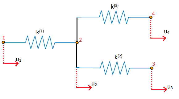
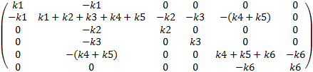
For this simple case the benefits of assembling the element stiffness matrices (as opposed to deriving the global stiffness matrix directly) aren’t immediately obvious. We consider therefore the following (more complex) system which contains 5 springs (elements) and 5 degrees of freedom (problems of practical interest can have tens or hundreds of thousands of degrees of freedom (and more!)). Since there are 5 degrees of freedom we know the matrix order is 5×5. We also know that it’s symmetrical, so it takes the form shown below:

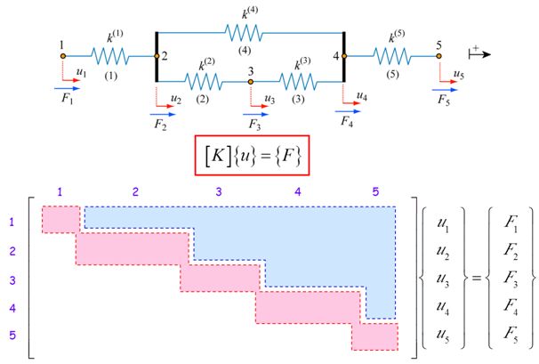
We want to populate the cells to generate the global stiffness matrix. From our observation of simpler systems, e.g. the two spring system above, the following rules emerge:

• The term in location ii consists of the sum of the direct stiffnesses of all the elements meeting at node i
• The term in location ij consists of the sum of the indirect stiffnesses relating to nodes i and j of all the elements joining node i to j
• Add a negative for reaction terms (–k_ij)
• Add a zero for node combinations that don’t interact

By following these rules, we can generate the global stiffness matrix:

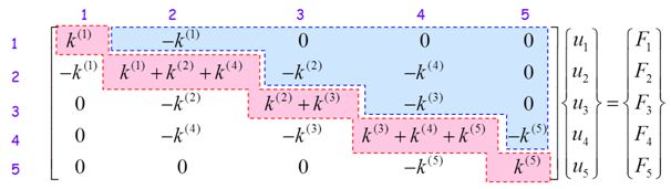
This type of assembly process is handled automatically by commercial FEM codes

Drag the springs into position and click 'Build matrix', then apply a force to node 5. You will then see the force equilibrium equations, the equivalent spring stiffness and the displacement at node 5.

Solving for (u)

The unknowns (degrees of freedom) in the spring systems presented are the displacements u_ij. Our global system of equations takes the following form:

To find {u} solve

\[{u}={F}{\left[ K \right]^{ - 1}}\;\;\;\;\;(22)\]

Recall that \(\left[ k \right]{\left[ k \right]^{ - 1}} = {\rm{I}} = \;\;{\rm{Identitiy\;Matrix}}\;\; = \;\left[ {\begin{array}{*{20}{c}} 1&0\\ 0&1 \end{array}} \right]\).

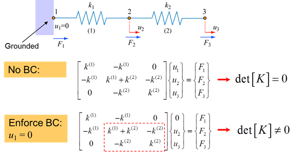
Recall also that, in order for a matrix to have an inverse, its determinant must be non-zero. If the determinant is zero, the matrix is said to be singular and no unique solution for Eqn.22 exists. For instance, consider once more the following spring system:

We know that the global stiffness matrix takes the following form \[\left[ {\begin{array}{*{20}{c}} {{k^1}}&{ - {k^1}}&0\\ { - {k^1}}&{{k^1} + {k^2}}&{ - {k^2}}\\ 0&{ - {k^2}}&{{k^2}} \end{array}} \right]\left\{ {\begin{array}{*{20}{c}} {{u_1}}\\ {{u_2}}\\ {{u_3}} \end{array}} \right\} = \;\left\{ {\begin{array}{*{20}{c}} {{F_1}}\\ {{F_2}}\\ {{F_3}} \end{array}} \right\} \;\;\;\;\; (23) \]

The determinant of [K] can be found from:

\[{\rm{det}}\left[ {\begin{array}{*{20}{c}} a&b&c\\ d&e&f\\ g&h&i \end{array}} \right] = \left( {aei + bfg + cdh} \right) - \left( {ceg + bdi + afh} \right) \;\;\;\;\;(24)\]

Such that:

\[ \left( {{k^1}\left( {{k^1} + {k^2}} \right){k^2} + 0 + 0} \right) - \left( {0 + \left( { - {k^1} - {k^1}{k^2}} \right) + \left( {{k^1} - {k^2} - {k^2}} \right)} \right) \;\;\;\;\;\;(25)\] \[{\rm{det}}\left[ K \right] = \left( {{k^1}^2{k^2} + {k^1}{k^2}^2} \right) - \left( {{k^1}^2{k^2} + {k^1}{k^2}^2} \right) = 0 \;\;\;\;\;\;(26) \]

Since the determinant of [K] is zero it is not invertible, but singular. There are no unique solutions and {u} cannot be found. If this is the case in your own model, then you are likely to receive an error message!

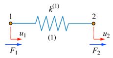
Enforcing Boundary Conditions

By enforcing boundary conditions, such as those depicted in the system below, [K] becomes invertible (non-singular) and we can solve for the reaction force F₁ and the unknown displacements u₂ and u₃, for known (applied) F₂ and F₃.

\[\left[ K \right] = \left[ {\begin{array}{*{20}{c}}{{k^1} + {k^2}}&{ - {k^2}}\\{ - {k^2}}&{{k^2}}\end{array}} \right] = \left[ {\begin{array}{*{20}{c}}a&b\\c&d\end{array}} \right] \;\;\;\;\;(27)\]

\[det\left[ K \right] = ad - cb \;\;\;\;\; (28) \]

\[det\left[ K \right] = \;\left( {{k^1} + {k^2}} \right){k^2} - {k^2}^2 = {k^1}{k^2} \ne 0 \;\;\;\;\; (29) \]

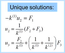
Unique solutions for \({F_1}\), \(\left\{ {{u_2}} \right\}\) and \(\left\{ {{u_3}} \right\}\) can now be found

\[ - {k^1}{u_2} = {F_1}\]

\[\left( {{k^1} + {k^2}} \right){u_2} - {k^2}{u_3} = {F_2} = {k^1}{u_2} + {k^2}{u_2} - {k^2}{u_3}\]

\[ - {k^2}{u_2} + {k^2}{u_3} = {F_3}\]

In this instance we solved three equations for three unknowns. In problems of practical interest the order of \(\left[ K \right]\) is often very large and we can have thousands of unknowns. It then becomes impractical to solve for \(\left\{ u \right\}\) by direct inversion of the global stiffness matrix. We can instead use Gauss elimination which is much more suitable for solving systems of linear equations with thousands of unknowns.

Gauss Elimination

We have a system of equations

\[x - 3y + z = 4 \;\;\;\;\; \rm{(30)} \]

\[2x - 8y + 8z = - 2 \;\;\;\;\; \rm{(31)} \]

\[ - 6x + 3y - 15z = 9 \;\;\;\;\; \rm{(32)} \]

when expressed in augmented matrix form

\[\left[ {\left. {\begin{array}{*{20}{c}}1&{ - 3}&1\\2&{ - 8}&8\\{ - 6}&3&{ - 15}\end{array}} \right|\begin{array}{*{20}{c}}4\\{ - 2}\\9\end{array}} \right] \;\;\;\;\; \rm{(33)} \]

We wish to create a matrix of the following form

\[\left[ {\left. {\begin{array}{*{20}{c}}{11}&{12}&{13}\\0&{22}&{23}\\0&0&{33}\end{array}} \right|\begin{array}{*{20}{c}}1\\2\\3\end{array}} \right] \;\;\;\;\; \rm{(34)} \]

Where the terms below the direct terms are zero. We need to eliminate some of the unknowns by solving the system of simultaneous equations. To eliminate x from row 2 (where R denotes the row)

-2(R1) + R2       (35)

\[ - 2\left( {x - 3y + z} \right) + \left( {2x - 8y + 8z} \right) = - 10 \;\;\;\;\; \rm{(36)} \]

\[ - 2y + 6z = - 10 \;\;\;\;\; \rm{(37)} \]

So that

\[\left[ {\left. {\begin{array}{*{20}{c}}1&{ - 3}&1\\0&{ - 2}&6\\{ - 6}&3&{ - 15}\end{array}} \right|\begin{array}{*{20}{c}}4\\{ - 10}\\9\end{array}} \right] \;\;\;\;\; \rm{(38)} \]

To eliminate x from row 3

6(R1) + R3       (39)

\[6\left( {x - 3y + z} \right) + \left( { - 6x + 3y - 15z} \right) = 33 \;\;\;\;\; \rm{(40)} \]

\[ - 15y - 9z = 33 \;\;\;\;\; \rm{(41)} \]

\[\left[ {\left. {\begin{array}{*{20}{c}}1&{ - 3}&1\\0&{ - 2}&6\\0&{ - 15}&{ - 9}\end{array}} \right|\begin{array}{*{20}{c}}4\\{ - 10}\\{33}\end{array}} \right] \;\;\;\;\; \rm{(42)} \]

To eliminate y from row 2

R2/2

\[ - y + 3z = - 5 \;\;\;\;\; \rm{(43)} \]

\[\left[ {\left. {\begin{array}{*{20}{c}}1&{ - 3}&1\\0&{ - 1}&3\\0&{ - 15}&{ - 9}\end{array}} \right|\begin{array}{*{20}{c}}4\\{ - 5}\\{33}\end{array}} \right] \;\;\;\;\; \rm{(44)} \]

To eliminate y from row 3

R3/3

\[ - 5y - 3z = - 11 \;\;\;\;\; \rm{(45)} \]

\[\left[ {\left. {\begin{array}{*{20}{c}}1&{ - 3}&1\\0&{ - 1}&3\\0&{ - 5}&{ - 3}\end{array}} \right|\begin{array}{*{20}{c}}4\\{ - 5}\\{11}\end{array}} \right] \;\;\;\;\; \rm{(46)} \]

And then

-5(R2) + R3       (47)

\[ - 5\left( { - y + 3z} \right) + \left( { - 5y - 3z} \right) = 36 \;\;\;\;\; \rm{(48)} \]

\[ - 18z = 36 \;\;\;\;\; \rm{(49)} \]

\[\left[ {\left. {\begin{array}{*{20}{c}}1&{ - 3}&1\\0&{ - 1}&3\\0&0&{ - 18}\end{array}} \right|\begin{array}{*{20}{c}}4\\{ - 5}\\{36}\end{array}} \right] \;\;\;\;\; \rm{(50)} \]

\[ - 2 = z \;\;\;\;\; \rm{(51)} \]

Substituting z = -2 back in to R2 gives y = -1

Substituting y = -1 and z = -2 back in to R1 gives x = 3

This process of progressively solving for the unknowns is called back substitution.

Interpolation/Basis/Shape Functions

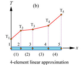
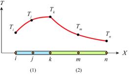
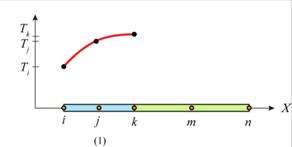
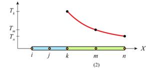
Consider the temperature distribution along the one-dimensional fin in Fig.1.

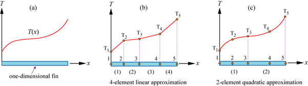
A one-dimensional continuous temperature distribution with an infinite number of unknowns is shown in (a). The fin is discretised in (b) – i.e. divided into 4 subdomains (or elements). The nodes are numbered consecutively from left to right, as are the elements. The elements are first order elements; the interpolation scheme between the nodes is therefore linear. Note that there are only 5 nodes for this system, since the internal nodes are shared between the elements. Since we are only solving for temperature, there are only 5 degrees of freedom in this model of the continuous system. It should be clear that a better approximation for T(x) would be obtained if the number of elements was increased (i.e. if the element lengths were reduced). It is also apparent that the nodes should be placed closer together in regions where the temperature (or any other unknown solution) changes rapidly. It is useful also to place a node wherever a step change in temperature is expected and where a numerical value of the temperature is needed. It is good practice to continue to increase the number of nodes until a converged solution is reached.

In (c), the fin has been divided into two subdomains – elements 1 and 2. However, in this instance we have chosen to use a second order (quadratic) element. These elements contain ‘midside’ nodes as shown, and the interpolation between the nodes is quadratic which permits a much closer approximation to the real system. For this model system there are still just 5 degrees of freedom. However, the analysis takes longer for (c) than it does for (b) because the quadratic interpolation (which calculates the temperature at locations between the nodes) is more demanding than the corresponding linear case.

(There is often a trade-off between a high number of first order elements requiring little computation and a smaller number of second order elements requiring more heavy computation to be made, which affects both the analysis time and the solution accuracy. The choice depends to a large extent on the problem being solved.)

1D first order shape functions

We can use (for instance) the direct stiffness method to compute degrees of freedom at the element nodes. However, we are also interested in the value of the solution at positions inside the element. To calculate values at positions other than the nodes we interpolate between the nodes using shape functions.

A one-dimensional element with length L is shown below. It has two nodes, one at each end, denoted i and j, and known nodal temperatures T_i and T_j. We can deduce automatically that the element is first order (linear) since it contains no ‘midside’ nodes.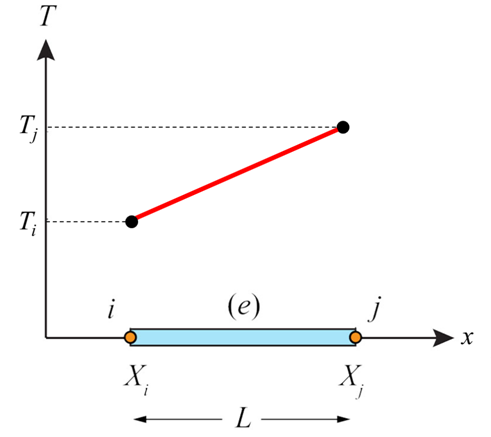

One dimensional linear element with temperature degrees of freedom

We need to derive a function to compute values of the temperature at locations between the nodes. This interpolation function is called the shape function. We demonstrate its derivation for a 1-dimensional linear element here. Note that, for linear elements, the polynomial inerpolation function is first order. If the element was second order, the polynomial function would be second order (quadratic), and so on.

Since the element is first order, the temperature varies linearly between the nodes and the equation for T is:

\[ T\left( x \right) = a + bx \;\;\;\;\; \rm{(1)} \]

We can therefore write:

\[ {T_i} = a + b{X_i} \;\;\;\;\; \rm{(2)} \]

\[ {T_j} = a + b{X_j} \;\;\;\;\; \rm{(3)} \]

which are simultaneous. To determine the coefficients \(a\) and \(b\):

\[ \frac{{{T_i} - a}}{{{X_i}}} = b \;\;\;\;\; \rm{(4)} \]

\[ \frac{{{T_j} - a}}{{{X_j}}} = b \;\;\;\;\; \rm{(5)} \]

\[ \frac{{{T_i} - a}}{{{X_i}}} = \;\frac{{{T_j} - a}}{{{X_j}}} \;\;\;\;\; \rm{(6)} \]

\[ \left( {{T_i} - a} \right){X_j} = \;\left( {{T_j} - a} \right){X_i} \;\;\;\;\; \rm{(7)} \]

\[ {T_i}{X_j} - a{X_j} = \;{T_j}{X_i} - a{X_i} \;\;\;\;\; \rm{(8)} \]

\[ {T_i}{X_j} - {T_j}{X_i} = \;a\left( {{X_j} - {X_i}} \right) \;\;\;\;\; \rm{(9)} \]

\[ \frac{{{T_i}{X_j} - {T_j}{X_i}}}{{\left( {{X_j} - {X_i}} \right)}} = \;a \;\;\;\;\; \rm{(10)} \]

\[ \frac{{{T_i}{X_j} - {T_j}{X_i}}}{L} = \;a \;\;\;\;\; \rm{(11)} \]

and

\[ {T_i} - b{X_i} = a \;\;\;\;\; \rm{(12)} \]

\[ {T_j} - b{X_j} = a \;\;\;\;\; \rm{(13)} \]

\[ {T_i} - b{X_i} = {T_j} - b{X_j} \;\;\;\;\; \rm{(14)} \]

\[ b{X_j} - b{X_i} = {T_j} - {T_i} \;\;\;\;\; \rm{(15)} \]

\[ b\left( {{X_j} - {X_i}} \right) = {T_j} - {T_i} \;\;\;\;\; \rm{(16)} \]

\[ b = \frac{{{T_j} - {T_i}}}{{\left( {{X_j} - {X_i}} \right)}} \;\;\;\;\; \rm{(17)} \]

\[ b = \frac{{{T_j} - {T_i}}}{L} \;\;\;\;\; \rm{(18)} \]

Substitution of Eqns.11 and 18 into Eqn.1 yields:

\[ T\left( x \right) = \frac{{{T_i}{X_j} - {T_j}{X_i}}}{L} + \left( {\frac{{{T_j} - {T_i}}}{L}} \right)x \;\;\;\;\; \rm{(19)} \]

\[ T\left( x \right) = \frac{{{T_i}{X_j} - {T_j}{X_i}}}{L} + \frac{{{T_j}x - {T_i}x}}{L} \;\;\;\;\; \rm{(20)} \]

\[ T\left( x \right) = \frac{{{T_i}{X_j}}}{L} - \frac{{{T_j}{X_i}}}{L} + \frac{{{T_j}x}}{L} - \frac{{{T_i}x}}{L} \;\;\;\;\; \rm{(21)}\]

\[ T\left( x \right) = \frac{{{T_i}{X_j}}}{L} - \frac{{{T_i}x}}{L}{\rm{\;}} + \frac{{{T_j}x}}{L} - \frac{{{T_j}{X_i}}}{L} \;\;\;\;\; \rm{(22)}\]

\[ T\left( x \right) = {T_i}\left( {\frac{{{X_j} - x}}{L}} \right) + {T_j}\left( {\frac{{x - {X_i}}}{L}} \right) \;\;\;\;\; \rm{(23)}\]

It should be clear from Eqn.23 that the nodal temperature values are multiplied by linear functions of \(x\) – the shape functions. The functions are denoted by \(S\) with a subscript to indicate the node with which a specific shape function is associated. In the case presented:

\[ {S_i} = \;\left( {\frac{{{X_j} - x}}{L}} \right) \;\;\;\;\; \rm{(24)}\]

\[ {S_j} = \;\left( {\frac{{x - {X_i}}}{L}} \right) \;\;\;\;\; \rm{(25)}\]

And Eqn.23 becomes

\[ T\left( x \right) = {S_i}{T_i} + {S_j}{T_j} \;\;\;\;\; \rm{(26)}\]

In matrix form

\[ T_x^e = \left[ {\begin{array}{*{20}{c}}{{S_i}}&{{S_j}}\end{array}} \right]\left\{ {\begin{array}{*{20}{c}}{{T_i}}\\{{T_j}}\end{array}} \right\} \;\;\;\;\; \rm{(27)}\]

For the case shown below, calculate T at x = 3.3.

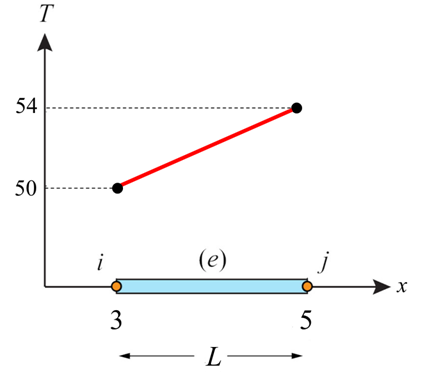\[T\left( {x = 3.3} \right) = {T_i}\left( {\frac{{{X_j} - x}}{L}} \right) + {T_j}\left( {\frac{{x - {X_i}}}{L}} \right)\] \[T\left( {x = 3.3} \right) = 50\left( {\frac{{5 - 3.3}}{2}} \right) + 54\left( {\frac{{3.3 - 3}}{2}} \right)\]

1-dimensional linear element with known nodal temperatures and positions

From inspection of Eqn.26 we can deduce that each shape function has a value of 1 at its own node and a value of zero at the other nodes. The sum of the shape functions sums to one. The shape functions are also first order, just as the original polynomial was. The shape functions would have been quadratic if the original polynomial had been quadratic.

A continuous, piecewise smooth equation for the one dimensional fin first shown above can be constructed by connecting the linear element equations. We know that the temperature at any point in any element can be found from the nodal temperatures T_i and the shape functions S_i. For the following system:

\[T_x^e = {S_i}{T_i} + {S_j}{T_j}\;\;\;\;\;\;\;{X_i} \le x \le {X_j} \;\;\;\;\; \rm{(28)} \]

	Node
Element #	i	j
1	1	2
2	2	3
3	3	4
4	4	5

\[T_x^1 = S_1^1{T_1} + S_2^1{T_2} \;\;\;\;\;\; S_1^1 = \frac{{{X_2} - x}}{{{X_2} - {X_1}}} \;\;\;\;\;\; S_2^1 = \frac{{x - {X_1}}}{{{X_2} - {X_1}}} \;\;\;\;\;\; {X_1} \le x \le {X_2} \;\;\;\;\;\; \rm{(29)} \]

\[T_x^2 = S_2^2{T_2} + S_3^2{T_3} \;\;\;\;\;\; S_2^2 = \frac{{{X_3} - x}}{{{X_3} - {X_2}}} \;\;\;\;\;\; S_3^2 = \frac{{x - {X_2}}}{{{X_3} - {X_2}}} \;\;\;\;\;\; {X_2} \le x \le {X_3} \;\;\;\;\;\; \rm{(30)} \]

\[T_x^3 = S_3^3{T_3} + S_4^3{T_4} \;\;\;\;\;\; S_3^3 = \frac{{{X_4} - x}}{{{X_4} - {X_3}}} \;\;\;\;\;\; S_4^3 = \frac{{x - {X_3}}}{{{X_4} - {X_3}}} \;\;\;\;\;\; {X_3} \le x \le {X_4} \;\;\;\;\;\; \rm{(31)} \]

\[T_x^4 = S_4^4{T_4} + S_5^4{T_5} \;\;\;\;\;\; S_4^4 = \frac{{{X_5} - x}}{{{X_5} - {X_4}}} \;\;\;\;\;\; S_4^3 = \frac{{x - {X_4}}}{{{X_5} - {X_4}}} \;\;\;\;\;\; {X_4} \le x \le {X_5} \;\;\;\;\;\; \rm{(32)} \]

\(S_2^1 \ne S_2^2\), \(S_3^2 \ne S_3^3\) and \(S_4^3 \ne S_4^4\)

The temperature gradient through an individual element \(\frac{{d{T^e}}}{{dx}}\) can be found from the derivative of Eqn.33

\[T_x^e = {T_i}\left( {\frac{{{X_j} - x}}{L}} \right) + {T_j}\left( {\frac{{x - {X_i}}}{L}} \right) \;\;\;\;\;\; \rm{(33)} \]

\[T_x^e = \frac{{{X_j}{T_i}}}{L} - \frac{{x{T_i}}}{L} + \frac{{x{T_j}}}{L} - \frac{{{X_i}{T_j}}}{L} \;\;\;\;\;\; \rm{(34)} \]

\[T_x^e = \frac{{x{T_j}}}{L} - \frac{{x{T_i}}}{L} + \frac{{{X_j}{T_i}}}{L} - \frac{{{X_i}{T_j}}}{L} \;\;\;\;\;\; \rm{(35)} \]

\[T_x^e = \frac{x}{L}\left( {{T_j} - {T_i}} \right) + \frac{1}{L}\left( {{X_j}{T_i} - {X_i}{T_j}} \right) \;\;\;\;\;\; \rm{(36)} \]

such that

\[\frac{{dT_x^e}}{{dx}} = \frac{{{T_j} - {T_i}}}{L} \;\;\;\;\;\; \rm{(37)} \]

We can check that our shape functions are correct by knowing that the shape function derivatives sum to zero.

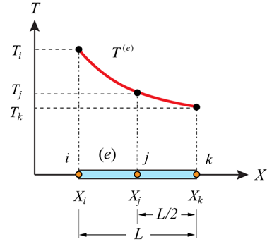
1D second order shape functions

A one-dimensional quadratic element is shown in Fig.4. We can deduce immediately that the element order is greater than one because the interpolation between the nodes in non-linear. We can determine from inspection that the element is quadratic (second order) because there’s a ‘midside’ node. We know therefore that the function approximating the solution is a second order polynomial:

\[T_x^e = a + bx + c{x^2} \;\;\;\;\; \rm{(38)} \]

The shape functions \({S_i}\) can be determined by solving Eqn.38 using known \({T_i}\) at known \({X_i}\) to give:

\[T_x^e = {S_i}{T_i} + {S_j}{T_j} + {S_k}{T_k}_j \;\;\;\;\; \rm{(39)} \] \[{S_i} = \frac{2}{{{L^2}}}\left( {x - {X_k}} \right)\left( {x - {X_j}} \right) \;\;\;\;\; \rm{(40)} \] \[{S_j} = \frac{{ - 4}}{{{L^2}}}\left( {x - {X_i}} \right)\left( {x - {X_k}} \right) \;\;\;\;\; \rm{(41)} \] \[{S_k} = \frac{2}{{{L^2}}}\left( {x - {X_i}} \right)\left( {x - {X_j}} \right) \;\;\;\;\; \rm{(42)} \]

Using the quadratic shape functions for a single element (Eqns.40-42), we can assemble a corresponding set of equations for a larger system:

	Nodes Element # i j k 1 i j k Nodes Element # i j k 2 k m n
	\[T_x^1 = \left[ {\begin{array}{*{20}{c}}{S_i^1}&{S_k^1}&{S_j^1}\end{array}} \right]\left\{ {\begin{array}{*{20}{c}}{{T_i}}\\{{T_k}}\\{{T_j}}\end{array}} \right\}\]
	\[T_x^2 = \left[ {\begin{array}{*{20}{c}}{S_k^2}&{S_m^2}&{S_n^2}\end{array}} \right]\left\{ {\begin{array}{*{20}{c}}{{T_k}}\\{{T_m}}\\{{T_n}}\end{array}} \right\}\]

\[T_x^1 = S_i^1{T_i} + S_j^1{T_j} + S_k^1{T_k} \;\;\;\;\; \rm{(43)} \] \[S_i^1 = \frac{2}{{{L^2}}}\left( {x - {X_k}} \right)\left( {x - {X_j}} \right)\] \[S_j^1 = \frac{{ - 4}}{{{L^2}}}\left( {x - {X_i}} \right)\left( {x - {X_k}} \right)\] \[S_k^1 = \frac{2}{{{L^2}}}\left( {x - {X_i}} \right)\left( {x - {X_j}} \right)\] \[T_x^2 = S_k^2{T_k} + S_m^2{T_m} + S_n^2{T_n} \;\;\;\;\; \rm{(44)} \] \[S_k^2 = \frac{2}{{{L^2}}}\left( {x - {X_n}} \right)\left( {x - {X_m}} \right)\] \[S_m^2 = \frac{{ - 4}}{{{L^2}}}\left( {x - {X_k}} \right)\left( {x - {X_n}} \right)\] \[S_n^2 = \frac{2}{{{L^2}}}\left( {x - {X_k}} \right)\left( {x - {X_m}} \right)\]

The element shape functions are stored within the element in commercial FE codes. The positions X_i are generated (and stored) when the mesh is created. Once the nodal degrees of freedom are known, the solution at any point between the nodes can be calculated using the (stored) element shape functions and the (known) nodal positions.

The order of the element and the number of elements in your geometric domain can have a strong effect on the accuracy of the solution. This is demonstrated in the following application which demonstrates how the number of elements (mesh density) can affect the accuracy of finite element model predictions. It compares the exact solution to the equation shown (which has an analytical solution) to predictions using the finite element method. In the application you can discretise (mesh) the "domain" using any number of elements between 1 and 20. The shape functions used are first order ones. The error between the exact solution and the FEM-predicted solution can be found by dragging the green cursor left and right through the domain.

Typical steps during FEM modelling

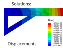
Consider a wall mounted bracket loaded uniformly along its length as in the figure below:

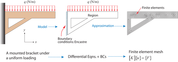
Wall mounted bracket

The geometry (field) is defined for us and is (relatively) complex. The boundary conditions are also defined and are:

• A uniform force per unit length (Neumann condition) along the upper edge
• Fixed x and y displacements along the clamped edge (Dirichlet condition)

It is apparent that the bracket will respond mechanically under the action of the applied load and a system of internal stresses will develop (to balance the applied load). To calculate the stresses that develop we must first mesh (discretise) the domain, assemble the global stiffness matrix [K], and then determine the nodal displacements {u} and resultant forces {F} using some iterative numerical technique (Gauss elimination, for instance). It is then a relatively trivial exercise to compute the nodal stresses from the nodal displacements and to find the solution between the nodes and within the elements using shape functions.

\(\underrightarrow {{\sigma _{ij}} = {C_{ijkl}}{\varepsilon _{kl}}}\)

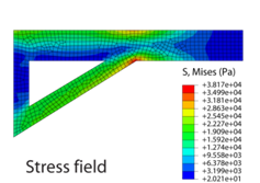
However, it is important to be aware that certain combinations of the specified number of elements (mesh density) and the specified element order can give rise to solutions that are highly inaccurate. It is highly advisable (and good practice) to perform a mesh sensitivity study, whereby the effect on the solution of successively finer meshes is analysed in order to eliminate any mesh sensitivity. The following application demonstrates this point:

The application below concerns the deflection of a CANTILEVER beam loaded at its end with an applied force. The width of the beam can be altered, although the beam length and beam depth are fixed constant. The beam can be made of either steel or aluminium and it can be loaded with a force of either 40 N or 80 N. The beam can then be meshed with either 2 elements through its thickness or 4 elements through its thickness. The elements can be either first or second order. For any combination chosen, a prediction of the beam deflection based on finite element calculations will be compared to predictions from (analytical) ordinary beam bending equations. It should become apparent that the error between the two decreases as the mesh density and element order are increased.

Summary

• You should now understand the basics of the finite element method
• You should be able to build a global stiffness matrix for a combination of 1-dimensional springs
• You should understand the importance of boundary conditions (including types of boundary conditions)
• You should be familiar with first and second order shape functions and you should be able to use these functions to calculate the value of a solution between nodes.
• You should understand and appreciate that the finite element method provides approximate solutions only, and that the accuracy of your solution will depend on element type and mesh density.

 

Questions

Quick questions

You should be able to answer these questions without too much difficulty after studying this TLP. If not, then you should go through it again!

1. Which is true? For second order elements:

   	a	The interpolation between the element nodes is linear
   	b	The shape function derivatives sum to 1
   	c	The solution between the nodes can be approximated using a second order polynomial
   	d	The solution between the nodes has no dependence on the solution at the nodes

2. Which is true? For first order elements:

   	a	The shape functions sum to 0
   	b	The shape function derivatives sum to 1
   	c	Field variables vary linearly between the element nodes
   	d	The elements contain midside nodes

3. Which is true? The error between an exact and finite element solution will always be reduced by:

   	a	Decreasing the element density
   	b	Increasing the element density
   	c	Increasing the element order
   	d	Decreasing the element order

4. If your finite element mesh contains 16 nodes, how many degrees of freedom are there in a coupled thermomechanical simulation:

   	a	64
   	b	48
   	c	24
   	d	16

5. In a structural mechanics analysis, what type of boundary condition is an applied pressure:

   	a	Dirichlet
   	b	Neumann
   	c	Robin
   	d	Dirichlet + Neumann

6. Discretise the following function using three equal length elements between \(0 \le x \le 6\). Assume the elements are linear (first order), and calculate \(\phi (x = 3.2)\) using the finite element method. Compare your answer to the exact solution.\[\phi = x(x - 3.5)(x + 3) + 30\]

7. Discretise the same function using six equal length elements and find \(\phi (x = 3.2)\) using the finite element method. Compare your answer to the exact solution and to the answer obtained using a three element discretisation.

8. Discretise the same function using three equal length but QUADRATIC elements. Calculate \(\phi (x = 3.2)\) and compare your answer to the ones obtained previously.

9. Using an equal length, 4-element discretisation of \(f(x) = 10 - {x^2}\), calculate \(f(x = 0.6)\) and the error between the finite element and exact solutions.

10. For the system of springs below, determine the global stiffness matrix.

11. A system of 1-dimensional springs has the following global stiffness matrix. Draw the system of springs.

Academic consultant: Dr James Dean, University of Cambridge and Double Precision Consultancy
Content development: Radu Bizga Nicolescu
Photography and video:
Web development: Lianne Sallows and David Brook

This DoITPoMS TLP was funded by the UK Centre for Materials Education and the Department of Materials Science and Metallurgy, University of Cambridge.