1D second order shape functions
A one-dimensional quadratic element is shown in Fig.4. We can deduce immediately that the element order is greater than one because the interpolation between the nodes in non-linear. We can determine from inspection that the element is quadratic (second order) because there’s a ‘midside’ node. We know therefore that the function approximating the solution is a second order polynomial:
\[T_x^e = a + bx + c{x^2} \;\;\;\;\; \rm{(38)} \]
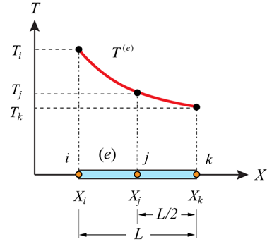
The shape functions \({S_i}\) can be determined by solving Eqn.38 using known \({T_i}\) at known \({X_i}\) to give:
\[T_x^e = {S_i}{T_i} + {S_j}{T_j} + {S_k}{T_k}_j \;\;\;\;\; \rm{(39)} \] \[{S_i} = \frac{2}{{{L^2}}}\left( {x - {X_k}} \right)\left( {x - {X_j}} \right) \;\;\;\;\; \rm{(40)} \] \[{S_j} = \frac{{ - 4}}{{{L^2}}}\left( {x - {X_i}} \right)\left( {x - {X_k}} \right) \;\;\;\;\; \rm{(41)} \] \[{S_k} = \frac{2}{{{L^2}}}\left( {x - {X_i}} \right)\left( {x - {X_j}} \right) \;\;\;\;\; \rm{(42)} \]
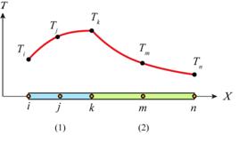
Using the quadratic shape functions for a single element (Eqns.40-42), we can assemble a corresponding set of equations for a larger system:
|
| ||||||||||||||||||||||||||||
|
\[T_x^1 = \left[ {\begin{array}{*{20}{c}}{S_i^1}&{S_k^1}&{S_j^1}\end{array}} \right]\left\{ {\begin{array}{*{20}{c}}{{T_i}}\\{{T_k}}\\{{T_j}}\end{array}} \right\}\] | ||||||||||||||||||||||||||||
|
\[T_x^2 = \left[ {\begin{array}{*{20}{c}}{S_k^2}&{S_m^2}&{S_n^2}\end{array}} \right]\left\{ {\begin{array}{*{20}{c}}{{T_k}}\\{{T_m}}\\{{T_n}}\end{array}} \right\}\] | ||||||||||||||||||||||||||||
\[T_x^1 = S_i^1{T_i} + S_j^1{T_j} + S_k^1{T_k} \;\;\;\;\; \rm{(43)} \] \[S_i^1 = \frac{2}{{{L^2}}}\left( {x - {X_k}} \right)\left( {x - {X_j}} \right)\] \[S_j^1 = \frac{{ - 4}}{{{L^2}}}\left( {x - {X_i}} \right)\left( {x - {X_k}} \right)\] \[S_k^1 = \frac{2}{{{L^2}}}\left( {x - {X_i}} \right)\left( {x - {X_j}} \right)\] \[T_x^2 = S_k^2{T_k} + S_m^2{T_m} + S_n^2{T_n} \;\;\;\;\; \rm{(44)} \] \[S_k^2 = \frac{2}{{{L^2}}}\left( {x - {X_n}} \right)\left( {x - {X_m}} \right)\] \[S_m^2 = \frac{{ - 4}}{{{L^2}}}\left( {x - {X_k}} \right)\left( {x - {X_n}} \right)\] \[S_n^2 = \frac{2}{{{L^2}}}\left( {x - {X_k}} \right)\left( {x - {X_m}} \right)\]
The element shape functions are stored within the element in commercial FE codes. The positions Xi are generated (and stored) when the mesh is created. Once the nodal degrees of freedom are known, the solution at any point between the nodes can be calculated using the (stored) element shape functions and the (known) nodal positions.
The order of the element and the number of elements in your geometric domain can have a strong effect on the accuracy of the solution. This is demonstrated in the following application which demonstrates how the number of elements (mesh density) can affect the accuracy of finite element model predictions. It compares the exact solution to the equation shown (which has an analytical solution) to predictions using the finite element method. In the application you can discretise (mesh) the "domain" using any number of elements between 1 and 20. The shape functions used are first order ones. The error between the exact solution and the FEM-predicted solution can be found by dragging the green cursor left and right through the domain.