Direct stiffness method and the global stiffness matrix
Although there are several finite element methods, we analyse the Direct Stiffness Method here, since it is a good starting point for understanding the finite element formulation. We consider first the simplest possible element – a 1-dimensional elastic spring which can accommodate only tensile and compressive forces. For the spring system shown, we accept the following conditions:
- Condition of Compatibility – connected ends (nodes) of adjacent springs have the same displacements
- Condition of Static Equilibrium – the resultant force at each node is zero
- Constitutive Relation – that describes how the material (spring) responds to the applied loads
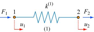
Model spring system
The constitutive relation can be obtained from the governing equation for an elastic bar loaded axially along its length:
\[\frac{d}{{du}}\left( {AE\frac{{\Delta l}}{{{l_0}}}} \right) + k = 0 \;\;\;\;\;(1)\]
\[\frac{{\Delta l}}{{{l_0}}} = \varepsilon \;\;\;\;\;(2) \]
\[\frac{d}{{du}}\left( {AE\varepsilon } \right) + k = 0 \;\;\;\;\;(3) \]
\[\frac{d}{{du}}\left( {A\sigma } \right) + k = 0 \;\;\;\;\;(4) \]
\[\frac{{dF}}{{du}} + k = 0 \;\;\;\;\;(5) \]
\[\frac{{dF}}{{du}} = - k \;\;\;\;\;(6) \]
\[dF = - kdu \;\;\;\;\;(7) \]
The spring stiffness equation relates the nodal displacements to the applied forces via the spring (element) stiffness. The minus sign denotes that the force is a restoring one, but from here on in we use the scalar version of Eqn.7.
Derivation of the Stiffness Matrix for a Single Spring Element
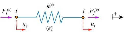
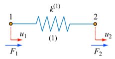
From inspection, we can see that there are two degrees of freedom in this model, ui and uj. We can write the force equilibrium equations:
\[{k^{\left( e \right)}}{u_i} - {k^{\left( e \right)}}{u_j} = F_i^{\left( e \right)} \;\;\;\;\;(8) \] \[ - {k^{\left( e \right)}}{u_i} + {k^{\left( e \right)}}{u_j} = F_j^{\left( e \right)} \;\;\;\;\;(9) \]
In matrix form
\[\left[ {\begin{array}{*{20}{c}}{{k^e}}&{ - {k^e}}\\{ - {k^e}}&{{k^e}}\end{array}} \right]\left\{ {\begin{array}{*{20}{c}}{{u_i}}\\{{u_j}}\end{array}} \right\} = \;\left\{ {\begin{array}{*{20}{c}}{F_i^{\left( e \right)}}\\{F_j^{\left( e \right)}}\end{array}} \right\} \;\;\;\;\;(10) \]
The order of the matrix is [2×2] because there are 2 degrees of freedom. Note also that the matrix is symmetrical. The ‘element’ stiffness relation is:
\[[{K^{(e)}}]\{ {u^{(e)}}\} = \{ {F^{(e)}}\} \;\;\;\;\;(11) \]
Where Κ(e) is the element stiffness matrix, u(e) the nodal displacement vector and F(e) the nodal force vector. (The element stiffness relation is important because it can be used as a building block for more complex systems. An example of this is provided later.)
Derivation of a Global Stiffness Matrix
For a more complex spring system, a ‘global’ stiffness matrix is required – i.e. one that describes the behaviour of the complete system, and not just the individual springs.
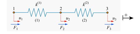
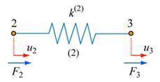
From inspection, we can see that there are two springs (elements) and three degrees of freedom in this model, u1, u2 and u3. As with the single spring model above, we can write the force equilibrium equations:
\[{k^1}{u_1} - {k^1}{u_2} = {F_1} \;\;\;\;\;(12) \]
\[ - {k^1}{u_1} + \left( {{k^1} + {k^2}} \right){u_2} - {k^2}{u_3} = {F_2} \;\;\;\;\;(13) \]
\[{k^2}{u_3} - {k^2}{u_2} = {F_3 \;\;\;\;\;(14) }\]
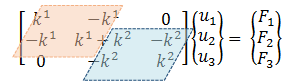
In matrix form \[\left[ {\begin{array}{*{20}{c}} {{k^1}}&{ - {k^1}}&0\\ { - {k^1}}&{{k^1} + {k^2}}&{ - {k^2}}\\ 0&{ - {k^2}}&{{k^2}} \end{array}} \right]\left\{ {\begin{array}{*{20}{c}} {{u_1}}\\ {{u_2}}\\ {{u_3}} \end{array}} \right\} = \;\left\{ {\begin{array}{*{20}{c}} {{F_1}}\\ {{F_2}}\\ {{F_3}} \end{array}} \right\} \;\;\;\;\;(15) \]
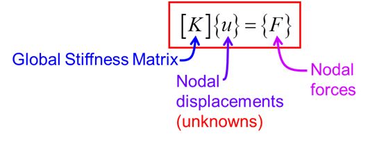
The ‘global’ stiffness relation is written in Eqn.16, which we distinguish from the ‘element’ stiffness relation in Eqn.11. \[\left[ K \right]\left\{ u \right\} = \;\left\{ F \right\} \;\;\;\;\;(16) \]
Note the shared k1 and k2 at k22 because of the compatibility condition at u2. We return to this important feature later on.
Assembling the Global Stiffness Matrix from the Element Stiffness Matrices
Although it isn’t apparent for the simple two-spring model above, generating the global stiffness matrix (directly) for a complex system of springs is impractical. A more efficient method involves the assembly of the individual element stiffness matrices. For instance, if you take the 2-element spring system shown,
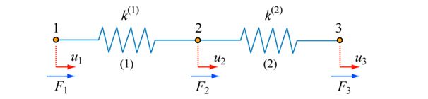
split it into its component parts in the following way
and derive the force equilibrium equations \[{k^1}{u_1} - {k^1}{u_2} = {F_1} \;\;\;\;\;(17) \] \[{k^1}{u_2} - {k^1}{u_1} = {k^2}{u_2} - {k^2}{u_3} = {F_2} \;\;\;\;\;(18) \] \[{k^2}{u_3} - {k^2}{u_2} = {F_3} \;\;\;\;\;(19) \] then the individual element stiffness matrices are: \[\left[ {\begin{array}{*{20}{c}} {{k^1}}&{ - {k^1}}\\ { - {k^1}}&{{k^1}} \end{array}} \right]\left\{ {\begin{array}{*{20}{c}} {{u_1}}\\ {{u_2}} \end{array}} \right\} = \;\left\{ {\begin{array}{*{20}{c}} {{F_1}}\\ {{F_2}} \end{array}} \right\}\;\;{\rm{and}}\;\;\left[ {\begin{array}{*{20}{c}} {{k^2}}&{ - {k^2}}\\ { - {k^2}}&{{k^2}} \end{array}} \right]\left\{ {\begin{array}{*{20}{c}} {{u_2}}\\ {{u_3}} \end{array}} \right\} = \;\left\{ {\begin{array}{*{20}{c}} {{F_2}}\\ {{F_3}} \end{array}} \right\} \;\;\;\;\;(20) \]
such that the global stiffness matrix is the same as that derived directly in Eqn.15:
(Note that, to create the global stiffness matrix by assembling the element stiffness matrices, k22 is given by the sum of the direct stiffnesses acting on node 2 – which is the compatibility criterion. Note also that the indirect cells kij are either zero (no load transfer between nodes i and j), or negative to indicate a reaction force.)
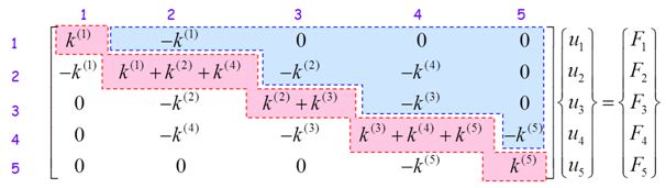
For this simple case the benefits of assembling the element stiffness matrices (as opposed to deriving the global stiffness matrix directly) aren’t immediately obvious. We consider therefore the following (more complex) system which contains 5 springs (elements) and 5 degrees of freedom (problems of practical interest can have tens or hundreds of thousands of degrees of freedom (and more!)). Since there are 5 degrees of freedom we know the matrix order is 5×5. We also know that it’s symmetrical, so it takes the form shown below:
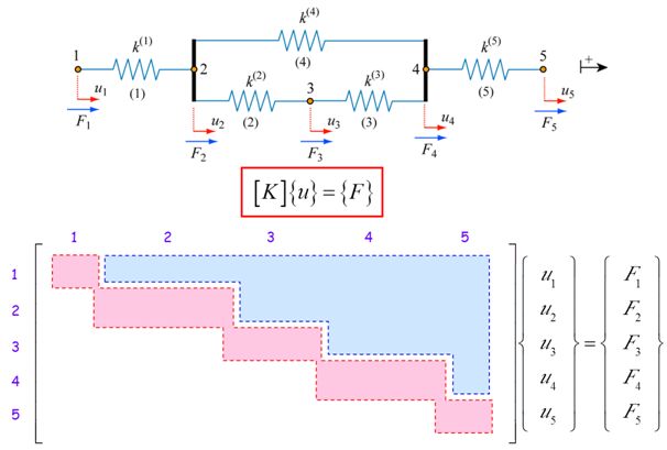
We want to populate the cells to generate the global stiffness matrix. From our observation of simpler systems, e.g. the two spring system above, the following rules emerge:
- The term in location ii consists of the sum of the direct stiffnesses of all the elements meeting at node i
- The term in location ij consists of the sum of the indirect stiffnesses relating to nodes i and j of all the elements joining node i to j
- Add a negative for reaction terms (–kij)
- Add a zero for node combinations that don’t interact
By following these rules, we can generate the global stiffness matrix:
This type of assembly process is handled automatically by commercial FEM codes
Drag the springs into position and click 'Build matrix', then apply a force to node 5. You will then see the force equilibrium equations, the equivalent spring stiffness and the displacement at node 5.
Solving for (u)
The unknowns (degrees of freedom) in the spring systems presented are the displacements uij. Our global system of equations takes the following form:
To find {u} solve
\[{u}={F}{\left[ K \right]^{ - 1}}\;\;\;\;\;(22)\]
Recall that \(\left[ k \right]{\left[ k \right]^{ - 1}} = {\rm{I}} = \;\;{\rm{Identitiy\;Matrix}}\;\; = \;\left[ {\begin{array}{*{20}{c}} 1&0\\ 0&1 \end{array}} \right]\).
Recall also that, in order for a matrix to have an inverse, its determinant must be non-zero. If the determinant is zero, the matrix is said to be singular and no unique solution for Eqn.22 exists. For instance, consider once more the following spring system:
We know that the global stiffness matrix takes the following form \[\left[ {\begin{array}{*{20}{c}} {{k^1}}&{ - {k^1}}&0\\ { - {k^1}}&{{k^1} + {k^2}}&{ - {k^2}}\\ 0&{ - {k^2}}&{{k^2}} \end{array}} \right]\left\{ {\begin{array}{*{20}{c}} {{u_1}}\\ {{u_2}}\\ {{u_3}} \end{array}} \right\} = \;\left\{ {\begin{array}{*{20}{c}} {{F_1}}\\ {{F_2}}\\ {{F_3}} \end{array}} \right\} \;\;\;\;\; (23) \]
The determinant of [K] can be found from:
\[{\rm{det}}\left[ {\begin{array}{*{20}{c}} a&b&c\\ d&e&f\\ g&h&i \end{array}} \right] = \left( {aei + bfg + cdh} \right) - \left( {ceg + bdi + afh} \right) \;\;\;\;\;(24)\]
Such that:
\[ \left( {{k^1}\left( {{k^1} + {k^2}} \right){k^2} + 0 + 0} \right) - \left( {0 + \left( { - {k^1} - {k^1}{k^2}} \right) + \left( {{k^1} - {k^2} - {k^2}} \right)} \right) \;\;\;\;\;\;(25)\] \[{\rm{det}}\left[ K \right] = \left( {{k^1}^2{k^2} + {k^1}{k^2}^2} \right) - \left( {{k^1}^2{k^2} + {k^1}{k^2}^2} \right) = 0 \;\;\;\;\;\;(26) \]
Since the determinant of [K] is zero it is not invertible, but singular. There are no unique solutions and {u} cannot be found. If this is the case in your own model, then you are likely to receive an error message!