1D first order shape functions
We can use (for instance) the direct stiffness method to compute degrees of freedom at the element nodes. However, we are also interested in the value of the solution at positions inside the element. To calculate values at positions other than the nodes we interpolate between the nodes using shape functions.
A one-dimensional element with length L is shown below. It has two nodes, one at each end, denoted i and j, and known nodal temperatures Ti and Tj. We can deduce automatically that the element is first order (linear) since it contains no ‘midside’ nodes.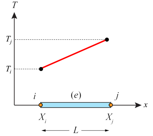
One dimensional linear element with temperature degrees of freedom
We need to derive a function to compute values of the temperature at locations between the nodes. This interpolation function is called the shape function. We demonstrate its derivation for a 1-dimensional linear element here. Note that, for linear elements, the polynomial inerpolation function is first order. If the element was second order, the polynomial function would be second order (quadratic), and so on.
Since the element is first order, the temperature varies linearly between the nodes and the equation for T is:
\[ T\left( x \right) = a + bx \;\;\;\;\; \rm{(1)} \]
We can therefore write:
\[ {T_i} = a + b{X_i} \;\;\;\;\; \rm{(2)} \]
\[ {T_j} = a + b{X_j} \;\;\;\;\; \rm{(3)} \]
which are simultaneous. To determine the coefficients \(a\) and \(b\):
\[ \frac{{{T_i} - a}}{{{X_i}}} = b \;\;\;\;\; \rm{(4)} \]
\[ \frac{{{T_j} - a}}{{{X_j}}} = b \;\;\;\;\; \rm{(5)} \]
\[ \frac{{{T_i} - a}}{{{X_i}}} = \;\frac{{{T_j} - a}}{{{X_j}}} \;\;\;\;\; \rm{(6)} \]
\[ \left( {{T_i} - a} \right){X_j} = \;\left( {{T_j} - a} \right){X_i} \;\;\;\;\; \rm{(7)} \]
\[ {T_i}{X_j} - a{X_j} = \;{T_j}{X_i} - a{X_i} \;\;\;\;\; \rm{(8)} \]
\[ {T_i}{X_j} - {T_j}{X_i} = \;a\left( {{X_j} - {X_i}} \right) \;\;\;\;\; \rm{(9)} \]
\[ \frac{{{T_i}{X_j} - {T_j}{X_i}}}{{\left( {{X_j} - {X_i}} \right)}} = \;a \;\;\;\;\; \rm{(10)} \]
\[ \frac{{{T_i}{X_j} - {T_j}{X_i}}}{L} = \;a \;\;\;\;\; \rm{(11)} \]
and
\[ {T_i} - b{X_i} = a \;\;\;\;\; \rm{(12)} \]
\[ {T_j} - b{X_j} = a \;\;\;\;\; \rm{(13)} \]
\[ {T_i} - b{X_i} = {T_j} - b{X_j} \;\;\;\;\; \rm{(14)} \]
\[ b{X_j} - b{X_i} = {T_j} - {T_i} \;\;\;\;\; \rm{(15)} \]
\[ b\left( {{X_j} - {X_i}} \right) = {T_j} - {T_i} \;\;\;\;\; \rm{(16)} \]
\[ b = \frac{{{T_j} - {T_i}}}{{\left( {{X_j} - {X_i}} \right)}} \;\;\;\;\; \rm{(17)} \]
\[ b = \frac{{{T_j} - {T_i}}}{L} \;\;\;\;\; \rm{(18)} \]
Substitution of Eqns.11 and 18 into Eqn.1 yields:
\[ T\left( x \right) = \frac{{{T_i}{X_j} - {T_j}{X_i}}}{L} + \left( {\frac{{{T_j} - {T_i}}}{L}} \right)x \;\;\;\;\; \rm{(19)} \]
\[ T\left( x \right) = \frac{{{T_i}{X_j} - {T_j}{X_i}}}{L} + \frac{{{T_j}x - {T_i}x}}{L} \;\;\;\;\; \rm{(20)} \]
\[ T\left( x \right) = \frac{{{T_i}{X_j}}}{L} - \frac{{{T_j}{X_i}}}{L} + \frac{{{T_j}x}}{L} - \frac{{{T_i}x}}{L} \;\;\;\;\; \rm{(21)}\]
\[ T\left( x \right) = \frac{{{T_i}{X_j}}}{L} - \frac{{{T_i}x}}{L}{\rm{\;}} + \frac{{{T_j}x}}{L} - \frac{{{T_j}{X_i}}}{L} \;\;\;\;\; \rm{(22)}\]
\[ T\left( x \right) = {T_i}\left( {\frac{{{X_j} - x}}{L}} \right) + {T_j}\left( {\frac{{x - {X_i}}}{L}} \right) \;\;\;\;\; \rm{(23)}\]
It should be clear from Eqn.23 that the nodal temperature values are multiplied by linear functions of \(x\) – the shape functions. The functions are denoted by \(S\) with a subscript to indicate the node with which a specific shape function is associated. In the case presented:
\[ {S_i} = \;\left( {\frac{{{X_j} - x}}{L}} \right) \;\;\;\;\; \rm{(24)}\]
\[ {S_j} = \;\left( {\frac{{x - {X_i}}}{L}} \right) \;\;\;\;\; \rm{(25)}\]
And Eqn.23 becomes
\[ T\left( x \right) = {S_i}{T_i} + {S_j}{T_j} \;\;\;\;\; \rm{(26)}\]
In matrix form
\[ T_x^e = \left[ {\begin{array}{*{20}{c}}{{S_i}}&{{S_j}}\end{array}} \right]\left\{ {\begin{array}{*{20}{c}}{{T_i}}\\{{T_j}}\end{array}} \right\} \;\;\;\;\; \rm{(27)}\]
For the case shown below, calculate T at x = 3.3.
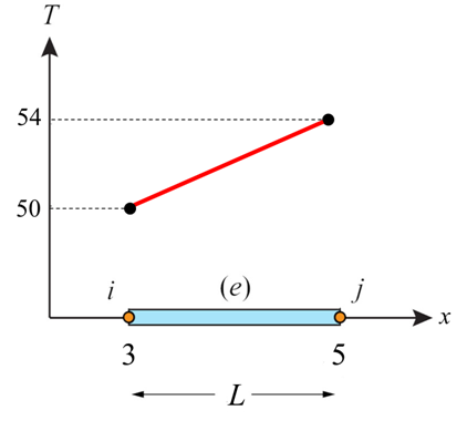 |
\[T\left( {x = 3.3} \right) = {T_i}\left( {\frac{{{X_j} - x}}{L}} \right) + {T_j}\left( {\frac{{x - {X_i}}}{L}} \right)\] \[T\left( {x = 3.3} \right) = 50\left( {\frac{{5 - 3.3}}{2}} \right) + 54\left( {\frac{{3.3 - 3}}{2}} \right)\] |
1-dimensional linear element with known nodal temperatures and positions
From inspection of Eqn.26 we can deduce that each shape function has a value of 1 at its own node and a value of zero at the other nodes. The sum of the shape functions sums to one. The shape functions are also first order, just as the original polynomial was. The shape functions would have been quadratic if the original polynomial had been quadratic.
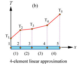
A continuous, piecewise smooth equation for the one dimensional fin first shown above can be constructed by connecting the linear element equations. We know that the temperature at any point in any element can be found from the nodal temperatures Ti and the shape functions Si. For the following system:
\[T_x^e = {S_i}{T_i} + {S_j}{T_j}\;\;\;\;\;\;\;{X_i} \le x \le {X_j} \;\;\;\;\; \rm{(28)} \]
Node |
||
Element # |
i |
j |
1 |
1 |
2 |
2 |
2 |
3 |
3 |
3 |
4 |
4 |
4 |
5 |
\[T_x^1 = S_1^1{T_1} + S_2^1{T_2} \;\;\;\;\;\; S_1^1 = \frac{{{X_2} - x}}{{{X_2} - {X_1}}} \;\;\;\;\;\; S_2^1 = \frac{{x - {X_1}}}{{{X_2} - {X_1}}} \;\;\;\;\;\; {X_1} \le x \le {X_2} \;\;\;\;\;\; \rm{(29)} \]
\[T_x^2 = S_2^2{T_2} + S_3^2{T_3} \;\;\;\;\;\; S_2^2 = \frac{{{X_3} - x}}{{{X_3} - {X_2}}} \;\;\;\;\;\; S_3^2 = \frac{{x - {X_2}}}{{{X_3} - {X_2}}} \;\;\;\;\;\; {X_2} \le x \le {X_3} \;\;\;\;\;\; \rm{(30)} \]
\[T_x^3 = S_3^3{T_3} + S_4^3{T_4} \;\;\;\;\;\; S_3^3 = \frac{{{X_4} - x}}{{{X_4} - {X_3}}} \;\;\;\;\;\; S_4^3 = \frac{{x - {X_3}}}{{{X_4} - {X_3}}} \;\;\;\;\;\; {X_3} \le x \le {X_4} \;\;\;\;\;\; \rm{(31)} \]
\[T_x^4 = S_4^4{T_4} + S_5^4{T_5} \;\;\;\;\;\; S_4^4 = \frac{{{X_5} - x}}{{{X_5} - {X_4}}} \;\;\;\;\;\; S_4^3 = \frac{{x - {X_4}}}{{{X_5} - {X_4}}} \;\;\;\;\;\; {X_4} \le x \le {X_5} \;\;\;\;\;\; \rm{(32)} \]
\(S_2^1 \ne S_2^2\), \(S_3^2 \ne S_3^3\) and \(S_4^3 \ne S_4^4\)
The temperature gradient through an individual element \(\frac{{d{T^e}}}{{dx}}\) can be found from the derivative of Eqn.33
\[T_x^e = {T_i}\left( {\frac{{{X_j} - x}}{L}} \right) + {T_j}\left( {\frac{{x - {X_i}}}{L}} \right) \;\;\;\;\;\; \rm{(33)} \]
\[T_x^e = \frac{{{X_j}{T_i}}}{L} - \frac{{x{T_i}}}{L} + \frac{{x{T_j}}}{L} - \frac{{{X_i}{T_j}}}{L} \;\;\;\;\;\; \rm{(34)} \]
\[T_x^e = \frac{{x{T_j}}}{L} - \frac{{x{T_i}}}{L} + \frac{{{X_j}{T_i}}}{L} - \frac{{{X_i}{T_j}}}{L} \;\;\;\;\;\; \rm{(35)} \]
\[T_x^e = \frac{x}{L}\left( {{T_j} - {T_i}} \right) + \frac{1}{L}\left( {{X_j}{T_i} - {X_i}{T_j}} \right) \;\;\;\;\;\; \rm{(36)} \]
such that
\[\frac{{dT_x^e}}{{dx}} = \frac{{{T_j} - {T_i}}}{L} \;\;\;\;\;\; \rm{(37)} \]
We can check that our shape functions are correct by knowing that the shape function derivatives sum to zero.